
diff options
| author | 2018-08-27 11:57:42 -0700 | |
|---|---|---|
| committer | 2018-08-27 12:01:50 -0700 | |
| commit | 6c2bf6576321ad53ff1eb6d66b6efae2c93ef4e0 (patch) | |
| tree | eda82ca98d1ac04718c14c086e6221bd8d787b30 /tensorflow/docs_src | |
| parent | abc8452394aeeecc1f3fef27f7098a5924bdd0e9 (diff) | |
Moved tensorflow/docs_src to https://github.com/tensorflow/docs
PiperOrigin-RevId: 210405729
Diffstat (limited to 'tensorflow/docs_src')
150 files changed, 3 insertions, 33942 deletions
diff --git a/tensorflow/docs_src/README.md b/tensorflow/docs_src/README.md new file mode 100644 index 0000000000..bcd896c5ba --- /dev/null +++ b/tensorflow/docs_src/README.md @@ -0,0 +1,3 @@ +# This directory has moved + +The new location is: https://github.com/tensorflow/docs/site/en diff --git a/tensorflow/docs_src/about/attribution.md b/tensorflow/docs_src/about/attribution.md deleted file mode 100644 index a4858b400a..0000000000 --- a/tensorflow/docs_src/about/attribution.md +++ /dev/null @@ -1,9 +0,0 @@ -# Attribution - -Please only use the TensorFlow name and marks when accurately referencing this -software distribution, and do not use our marks in a way that suggests you are -endorsed by or otherwise affiliated with Google. When referring to our marks, -please include the following attribution statement: "TensorFlow, the TensorFlow -logo and any related marks are trademarks of Google Inc." - - diff --git a/tensorflow/docs_src/about/bib.md b/tensorflow/docs_src/about/bib.md deleted file mode 100644 index 5593a3d95c..0000000000 --- a/tensorflow/docs_src/about/bib.md +++ /dev/null @@ -1,131 +0,0 @@ -# TensorFlow White Papers - -This document identifies white papers about TensorFlow. - -## Large-Scale Machine Learning on Heterogeneous Distributed Systems - -[Access this white paper.](https://static.googleusercontent.com/media/research.google.com/en//pubs/archive/45166.pdf) - -**Abstract:** TensorFlow is an interface for expressing machine learning -algorithms, and an implementation for executing such algorithms. -A computation expressed using TensorFlow can be -executed with little or no change on a wide variety of heterogeneous -systems, ranging from mobile devices such as phones -and tablets up to large-scale distributed systems of hundreds -of machines and thousands of computational devices such as -GPU cards. The system is flexible and can be used to express -a wide variety of algorithms, including training and inference -algorithms for deep neural network models, and it has been -used for conducting research and for deploying machine learning -systems into production across more than a dozen areas of -computer science and other fields, including speech recognition, -computer vision, robotics, information retrieval, natural -language processing, geographic information extraction, and -computational drug discovery. This paper describes the TensorFlow -interface and an implementation of that interface that -we have built at Google. The TensorFlow API and a reference -implementation were released as an open-source package under -the Apache 2.0 license in November, 2015 and are available at -www.tensorflow.org. - - -### In BibTeX format - -If you use TensorFlow in your research and would like to cite the TensorFlow -system, we suggest you cite this whitepaper. - -<pre> -@misc{tensorflow2015-whitepaper, -title={ {TensorFlow}: Large-Scale Machine Learning on Heterogeneous Systems}, -url={https://www.tensorflow.org/}, -note={Software available from tensorflow.org}, -author={ - Mart\'{\i}n~Abadi and - Ashish~Agarwal and - Paul~Barham and - Eugene~Brevdo and - Zhifeng~Chen and - Craig~Citro and - Greg~S.~Corrado and - Andy~Davis and - Jeffrey~Dean and - Matthieu~Devin and - Sanjay~Ghemawat and - Ian~Goodfellow and - Andrew~Harp and - Geoffrey~Irving and - Michael~Isard and - Yangqing Jia and - Rafal~Jozefowicz and - Lukasz~Kaiser and - Manjunath~Kudlur and - Josh~Levenberg and - Dandelion~Man\'{e} and - Rajat~Monga and - Sherry~Moore and - Derek~Murray and - Chris~Olah and - Mike~Schuster and - Jonathon~Shlens and - Benoit~Steiner and - Ilya~Sutskever and - Kunal~Talwar and - Paul~Tucker and - Vincent~Vanhoucke and - Vijay~Vasudevan and - Fernanda~Vi\'{e}gas and - Oriol~Vinyals and - Pete~Warden and - Martin~Wattenberg and - Martin~Wicke and - Yuan~Yu and - Xiaoqiang~Zheng}, - year={2015}, -} -</pre> - -Or in textual form: - -<pre> -Martín Abadi, Ashish Agarwal, Paul Barham, Eugene Brevdo, -Zhifeng Chen, Craig Citro, Greg S. Corrado, Andy Davis, -Jeffrey Dean, Matthieu Devin, Sanjay Ghemawat, Ian Goodfellow, -Andrew Harp, Geoffrey Irving, Michael Isard, Rafal Jozefowicz, Yangqing Jia, -Lukasz Kaiser, Manjunath Kudlur, Josh Levenberg, Dan Mané, Mike Schuster, -Rajat Monga, Sherry Moore, Derek Murray, Chris Olah, Jonathon Shlens, -Benoit Steiner, Ilya Sutskever, Kunal Talwar, Paul Tucker, -Vincent Vanhoucke, Vijay Vasudevan, Fernanda Viégas, -Oriol Vinyals, Pete Warden, Martin Wattenberg, Martin Wicke, -Yuan Yu, and Xiaoqiang Zheng. -TensorFlow: Large-scale machine learning on heterogeneous systems, -2015. Software available from tensorflow.org. -</pre> - - - -## TensorFlow: A System for Large-Scale Machine Learning - -[Access this white paper.](https://www.usenix.org/system/files/conference/osdi16/osdi16-abadi.pdf) - -**Abstract:** TensorFlow is a machine learning system that operates at -large scale and in heterogeneous environments. TensorFlow -uses dataflow graphs to represent computation, -shared state, and the operations that mutate that state. It -maps the nodes of a dataflow graph across many machines -in a cluster, and within a machine across multiple computational -devices, including multicore CPUs, generalpurpose -GPUs, and custom-designed ASICs known as -Tensor Processing Units (TPUs). This architecture gives -flexibility to the application developer: whereas in previous -“parameter server” designs the management of shared -state is built into the system, TensorFlow enables developers -to experiment with novel optimizations and training algorithms. -TensorFlow supports a variety of applications, -with a focus on training and inference on deep neural networks. -Several Google services use TensorFlow in production, -we have released it as an open-source project, and -it has become widely used for machine learning research. -In this paper, we describe the TensorFlow dataflow model -and demonstrate the compelling performance that TensorFlow -achieves for several real-world applications. - diff --git a/tensorflow/docs_src/about/index.md b/tensorflow/docs_src/about/index.md deleted file mode 100644 index c3c13ff329..0000000000 --- a/tensorflow/docs_src/about/index.md +++ /dev/null @@ -1,11 +0,0 @@ -# About TensorFlow - -This section provides a few documents about TensorFlow itself, -including the following: - - * [TensorFlow in Use](../about/uses.md), which provides a link to our model zoo and - lists some popular ways that TensorFlow is being used. - * [TensorFlow White Papers](../about/bib.md), which provides abstracts of white papers - about TensorFlow. - * [Attribution](../about/attribution.md), which specifies how to attribute and refer - to TensorFlow. diff --git a/tensorflow/docs_src/about/leftnav_files b/tensorflow/docs_src/about/leftnav_files deleted file mode 100644 index 63763b9d9c..0000000000 --- a/tensorflow/docs_src/about/leftnav_files +++ /dev/null @@ -1,4 +0,0 @@ -index.md -uses.md -bib.md -attribution.md diff --git a/tensorflow/docs_src/about/uses.md b/tensorflow/docs_src/about/uses.md deleted file mode 100644 index d3db98203e..0000000000 --- a/tensorflow/docs_src/about/uses.md +++ /dev/null @@ -1,68 +0,0 @@ -# TensorFlow In Use - -This page highlights TensorFlow models in real world use. - - -## Model zoo - -Please visit our collection of TensorFlow models in the -[TensorFlow Zoo](https://github.com/tensorflow/models). - -If you have built a model with TensorFlow, please consider publishing it in -the Zoo. - - -## Current uses - -This section describes some of the current uses of the TensorFlow system. - -> If you are using TensorFlow for research, for education, or for production -> usage in some product, we would love to add something about your usage here. -> Please feel free to [email us](mailto:usecases@tensorflow.org) a brief -> description of how you're using TensorFlow, or even better, send us a -> pull request to add an entry to this file. - -* **Deep Speech** -<ul> - <li>**Organization**: Mozilla</li> - <li> **Domain**: Speech Recognition</li> - <li> **Description**: A TensorFlow implementation motivated by Baidu's Deep Speech architecture.</li> - <li> **More info**: [GitHub Repo](https://github.com/mozilla/deepspeech)</li> -</ul> - -* **RankBrain** -<ul> - <li>**Organization**: Google</li> - <li> **Domain**: Information Retrieval</li> - <li> **Description**: A large-scale deployment of deep neural nets for search ranking on www.google.com.</li> - <li> **More info**: ["Google Turning Over Its Lucrative Search to AI Machines"](http://www.bloomberg.com/news/articles/2015-10-26/google-turning-its-lucrative-web-search-over-to-ai-machines)</li> -</ul> - -* **Inception Image Classification Model** -<ul> - <li> **Organization**: Google</li> - <li> **Description**: Baseline model and follow on research into highly accurate computer vision models, starting with the model that won the 2014 Imagenet image classification challenge</li> - <li> **More Info**: Baseline model described in [Arxiv paper](http://arxiv.org/abs/1409.4842)</li> -</ul> - -* **SmartReply** -<ul> - <li> **Organization**: Google</li> - <li> **Description**: Deep LSTM model to automatically generate email responses</li> - <li> **More Info**: [Google research blog post](http://googleresearch.blogspot.com/2015/11/computer-respond-to-this-email.html)</li> -</ul> - -* **Massively Multitask Networks for Drug Discovery** -<ul> - <li> **Organization**: Google and Stanford University</li> - <li> **Domain**: Drug discovery</li> - <li> **Description**: A deep neural network model for identifying promising drug candidates.</li> - <li> **More info**: [Arxiv paper](http://arxiv.org/abs/1502.02072)</li> -</ul> - -* **On-Device Computer Vision for OCR** -<ul> - <li> **Organization**: Google</li> - <li> **Description**: On-device computer vision model to do optical character recognition to enable real-time translation.</li> - <li> **More info**: [Google Research blog post](http://googleresearch.blogspot.com/2015/07/how-google-translate-squeezes-deep.html)</li> -</ul> diff --git a/tensorflow/docs_src/api_guides/cc/guide.md b/tensorflow/docs_src/api_guides/cc/guide.md deleted file mode 100644 index 2cd645afa7..0000000000 --- a/tensorflow/docs_src/api_guides/cc/guide.md +++ /dev/null @@ -1,301 +0,0 @@ -# C++ API - -Note: By default [tensorflow.org](https://www.tensorflow.org) shows docs for the -most recent stable version. The instructions in this doc require building from -source. You will probably want to build from the `master` version of tensorflow. -You should, as a result, be sure you are following the -[`master` version of this doc](https://www.tensorflow.org/versions/master/api_guides/cc/guide), -in case there have been any changes. - -Note: The C++ API is only designed to work with TensorFlow `bazel build`. -If you need a stand-alone option use the [C-api](../../install/install_c.md). -See [these instructions](https://docs.bazel.build/versions/master/external.html) -for details on how to include TensorFlow as a subproject (instead of building -your project from inside TensorFlow, as in this example). - -[TOC] - -TensorFlow's C++ API provides mechanisms for constructing and executing a data -flow graph. The API is designed to be simple and concise: graph operations are -clearly expressed using a "functional" construction style, including easy -specification of names, device placement, etc., and the resulting graph can be -efficiently run and the desired outputs fetched in a few lines of code. This -guide explains the basic concepts and data structures needed to get started with -TensorFlow graph construction and execution in C++. - -## The Basics - -Let's start with a simple example that illustrates graph construction and -execution using the C++ API. - -```c++ -// tensorflow/cc/example/example.cc - -#include "tensorflow/cc/client/client_session.h" -#include "tensorflow/cc/ops/standard_ops.h" -#include "tensorflow/core/framework/tensor.h" - -int main() { - using namespace tensorflow; - using namespace tensorflow::ops; - Scope root = Scope::NewRootScope(); - // Matrix A = [3 2; -1 0] - auto A = Const(root, { {3.f, 2.f}, {-1.f, 0.f} }); - // Vector b = [3 5] - auto b = Const(root, { {3.f, 5.f} }); - // v = Ab^T - auto v = MatMul(root.WithOpName("v"), A, b, MatMul::TransposeB(true)); - std::vector<Tensor> outputs; - ClientSession session(root); - // Run and fetch v - TF_CHECK_OK(session.Run({v}, &outputs)); - // Expect outputs[0] == [19; -3] - LOG(INFO) << outputs[0].matrix<float>(); - return 0; -} -``` - -Place this example code in the file `tensorflow/cc/example/example.cc` inside a -clone of the -TensorFlow -[github repository](http://www.github.com/tensorflow/tensorflow). Also place a -`BUILD` file in the same directory with the following contents: - -```python -load("//tensorflow:tensorflow.bzl", "tf_cc_binary") - -tf_cc_binary( - name = "example", - srcs = ["example.cc"], - deps = [ - "//tensorflow/cc:cc_ops", - "//tensorflow/cc:client_session", - "//tensorflow/core:tensorflow", - ], -) -``` - -Use `tf_cc_binary` rather than Bazel's native `cc_binary` to link in necessary -symbols from `libtensorflow_framework.so`. You should be able to build and run -the example using the following command (be sure to run `./configure` in your -build sandbox first): - -```shell -bazel run -c opt //tensorflow/cc/example:example -``` - -This example shows some of the important features of the C++ API such as the -following: - -* Constructing tensor constants from C++ nested initializer lists -* Constructing and naming of TensorFlow operations -* Specifying optional attributes to operation constructors -* Executing and fetching the tensor values from the TensorFlow session. - -We will delve into the details of each below. - -## Graph Construction - -### Scope - -`tensorflow::Scope` is the main data structure that holds the current state -of graph construction. A `Scope` acts as a handle to the graph being -constructed, as well as storing TensorFlow operation properties. The `Scope` -object is the first argument to operation constructors, and operations that use -a given `Scope` as their first argument inherit that `Scope`'s properties, such -as a common name prefix. Multiple `Scope`s can refer to the same graph, as -explained further below. - -Create a new `Scope` object by calling `Scope::NewRootScope`. This creates -some resources such as a graph to which operations are added. It also creates a -`tensorflow::Status` object which will be used to indicate errors encountered -when constructing operations. The `Scope` class has value semantics, thus, a -`Scope` object can be freely copied and passed around. - -The `Scope` object returned by `Scope::NewRootScope` is referred -to as the root scope. "Child" scopes can be constructed from the root scope by -calling various member functions of the `Scope` class, thus forming a hierarchy -of scopes. A child scope inherits all of the properties of the parent scope and -typically has one property added or changed. For instance, `NewSubScope(name)` -appends `name` to the prefix of names for operations created using the returned -`Scope` object. - -Here are some of the properties controlled by a `Scope` object: - -* Operation names -* Set of control dependencies for an operation -* Device placement for an operation -* Kernel attribute for an operation - -Please refer to `tensorflow::Scope` for the complete list of member functions -that let you create child scopes with new properties. - -### Operation Constructors - -You can create graph operations with operation constructors, one C++ class per -TensorFlow operation. Unlike the Python API which uses snake-case to name the -operation constructors, the C++ API uses camel-case to conform to C++ coding -style. For instance, the `MatMul` operation has a C++ class with the same name. - -Using this class-per-operation method, it is possible, though not recommended, -to construct an operation as follows: - -```c++ -// Not recommended -MatMul m(scope, a, b); -``` - -Instead, we recommend the following "functional" style for constructing -operations: - -```c++ -// Recommended -auto m = MatMul(scope, a, b); -``` - -The first parameter for all operation constructors is always a `Scope` object. -Tensor inputs and mandatory attributes form the rest of the arguments. - -For optional arguments, constructors have an optional parameter that allows -optional attributes. For operations with optional arguments, the constructor's -last optional parameter is a `struct` type called `[operation]:Attrs` that -contains data members for each optional attribute. You can construct such -`Attrs` in multiple ways: - -* You can specify a single optional attribute by constructing an `Attrs` object -using the `static` functions provided in the C++ class for the operation. For -example: - -```c++ -auto m = MatMul(scope, a, b, MatMul::TransposeA(true)); -``` - -* You can specify multiple optional attributes by chaining together functions - available in the `Attrs` struct. For example: - -```c++ -auto m = MatMul(scope, a, b, MatMul::TransposeA(true).TransposeB(true)); - -// Or, alternatively -auto m = MatMul(scope, a, b, MatMul::Attrs().TransposeA(true).TransposeB(true)); -``` - -The arguments and return values of operations are handled in different ways -depending on their type: - -* For operations that return single tensors, the object returned by - the operation object can be passed directly to other operation - constructors. For example: - -```c++ -auto m = MatMul(scope, x, W); -auto sum = Add(scope, m, bias); -``` - -* For operations producing multiple outputs, the object returned by the - operation constructor has a member for each of the outputs. The names of those - members are identical to the names present in the `OpDef` for the - operation. For example: - -```c++ -auto u = Unique(scope, a); -// u.y has the unique values and u.idx has the unique indices -auto m = Add(scope, u.y, b); -``` - -* Operations producing a list-typed output return an object that can - be indexed using the `[]` operator. That object can also be directly passed to - other constructors that expect list-typed inputs. For example: - -```c++ -auto s = Split(scope, 0, a, 2); -// Access elements of the returned list. -auto b = Add(scope, s[0], s[1]); -// Pass the list as a whole to other constructors. -auto c = Concat(scope, s, 0); -``` - -### Constants - -You may pass many different types of C++ values directly to tensor -constants. You may explicitly create a tensor constant by calling the -`tensorflow::ops::Const` function from various kinds of C++ values. For -example: - -* Scalars - -```c++ -auto f = Const(scope, 42.0f); -auto s = Const(scope, "hello world!"); -``` - -* Nested initializer lists - -```c++ -// 2x2 matrix -auto c1 = Const(scope, { {1, 2}, {2, 4} }); -// 1x3x1 tensor -auto c2 = Const(scope, { { {1}, {2}, {3} } }); -// 1x2x0 tensor -auto c3 = ops::Const(scope, { { {}, {} } }); -``` - -* Shapes explicitly specified - -```c++ -// 2x2 matrix with all elements = 10 -auto c1 = Const(scope, 10, /* shape */ {2, 2}); -// 1x3x2x1 tensor -auto c2 = Const(scope, {1, 2, 3, 4, 5, 6}, /* shape */ {1, 3, 2, 1}); -``` - -You may directly pass constants to other operation constructors, either by -explicitly constructing one using the `Const` function, or implicitly as any of -the above types of C++ values. For example: - -```c++ -// [1 1] * [41; 1] -auto x = MatMul(scope, { {1, 1} }, { {41}, {1} }); -// [1 2 3 4] + 10 -auto y = Add(scope, {1, 2, 3, 4}, 10); -``` - -## Graph Execution - -When executing a graph, you will need a session. The C++ API provides a -`tensorflow::ClientSession` class that will execute ops created by the -operation constructors. TensorFlow will automatically determine which parts of -the graph need to be executed, and what values need feeding. For example: - -```c++ -Scope root = Scope::NewRootScope(); -auto c = Const(root, { {1, 1} }); -auto m = MatMul(root, c, { {42}, {1} }); - -ClientSession session(root); -std::vector<Tensor> outputs; -session.Run({m}, &outputs); -// outputs[0] == {42} -``` - -Similarly, the object returned by the operation constructor can be used as the -argument to specify a value being fed when executing the graph. Furthermore, the -value to feed can be specified with the different kinds of C++ values used to -specify tensor constants. For example: - -```c++ -Scope root = Scope::NewRootScope(); -auto a = Placeholder(root, DT_INT32); -// [3 3; 3 3] -auto b = Const(root, 3, {2, 2}); -auto c = Add(root, a, b); -ClientSession session(root); -std::vector<Tensor> outputs; - -// Feed a <- [1 2; 3 4] -session.Run({ {a, { {1, 2}, {3, 4} } } }, {c}, &outputs); -// outputs[0] == [4 5; 6 7] -``` - -Please see the `tensorflow::Tensor` documentation for more information on how -to use the execution output. diff --git a/tensorflow/docs_src/api_guides/python/array_ops.md b/tensorflow/docs_src/api_guides/python/array_ops.md deleted file mode 100644 index ddeea80c56..0000000000 --- a/tensorflow/docs_src/api_guides/python/array_ops.md +++ /dev/null @@ -1,87 +0,0 @@ -# Tensor Transformations - -Note: Functions taking `Tensor` arguments can also take anything accepted by -`tf.convert_to_tensor`. - -[TOC] - -## Casting - -TensorFlow provides several operations that you can use to cast tensor data -types in your graph. - -* `tf.string_to_number` -* `tf.to_double` -* `tf.to_float` -* `tf.to_bfloat16` -* `tf.to_int32` -* `tf.to_int64` -* `tf.cast` -* `tf.bitcast` -* `tf.saturate_cast` - -## Shapes and Shaping - -TensorFlow provides several operations that you can use to determine the shape -of a tensor and change the shape of a tensor. - -* `tf.broadcast_dynamic_shape` -* `tf.broadcast_static_shape` -* `tf.shape` -* `tf.shape_n` -* `tf.size` -* `tf.rank` -* `tf.reshape` -* `tf.squeeze` -* `tf.expand_dims` -* `tf.meshgrid` - -## Slicing and Joining - -TensorFlow provides several operations to slice or extract parts of a tensor, -or join multiple tensors together. - -* `tf.slice` -* `tf.strided_slice` -* `tf.split` -* `tf.tile` -* `tf.pad` -* `tf.concat` -* `tf.stack` -* `tf.parallel_stack` -* `tf.unstack` -* `tf.reverse_sequence` -* `tf.reverse` -* `tf.reverse_v2` -* `tf.transpose` -* `tf.extract_image_patches` -* `tf.space_to_batch_nd` -* `tf.space_to_batch` -* `tf.required_space_to_batch_paddings` -* `tf.batch_to_space_nd` -* `tf.batch_to_space` -* `tf.space_to_depth` -* `tf.depth_to_space` -* `tf.gather` -* `tf.gather_nd` -* `tf.unique_with_counts` -* `tf.scatter_nd` -* `tf.dynamic_partition` -* `tf.dynamic_stitch` -* `tf.boolean_mask` -* `tf.one_hot` -* `tf.sequence_mask` -* `tf.dequantize` -* `tf.quantize_v2` -* `tf.quantized_concat` -* `tf.setdiff1d` - -## Fake quantization -Operations used to help train for better quantization accuracy. - -* `tf.fake_quant_with_min_max_args` -* `tf.fake_quant_with_min_max_args_gradient` -* `tf.fake_quant_with_min_max_vars` -* `tf.fake_quant_with_min_max_vars_gradient` -* `tf.fake_quant_with_min_max_vars_per_channel` -* `tf.fake_quant_with_min_max_vars_per_channel_gradient` diff --git a/tensorflow/docs_src/api_guides/python/check_ops.md b/tensorflow/docs_src/api_guides/python/check_ops.md deleted file mode 100644 index b52fdaa3ab..0000000000 --- a/tensorflow/docs_src/api_guides/python/check_ops.md +++ /dev/null @@ -1,19 +0,0 @@ -# Asserts and boolean checks - -* `tf.assert_negative` -* `tf.assert_positive` -* `tf.assert_proper_iterable` -* `tf.assert_non_negative` -* `tf.assert_non_positive` -* `tf.assert_equal` -* `tf.assert_integer` -* `tf.assert_less` -* `tf.assert_less_equal` -* `tf.assert_greater` -* `tf.assert_greater_equal` -* `tf.assert_rank` -* `tf.assert_rank_at_least` -* `tf.assert_type` -* `tf.is_non_decreasing` -* `tf.is_numeric_tensor` -* `tf.is_strictly_increasing` diff --git a/tensorflow/docs_src/api_guides/python/client.md b/tensorflow/docs_src/api_guides/python/client.md deleted file mode 100644 index fdd48e66dc..0000000000 --- a/tensorflow/docs_src/api_guides/python/client.md +++ /dev/null @@ -1,36 +0,0 @@ -# Running Graphs -[TOC] - -This library contains classes for launching graphs and executing operations. - -[This guide](../../guide/low_level_intro.md) has examples of how a graph -is launched in a `tf.Session`. - -## Session management - -* `tf.Session` -* `tf.InteractiveSession` -* `tf.get_default_session` - -## Error classes and convenience functions - -* `tf.OpError` -* `tf.errors.CancelledError` -* `tf.errors.UnknownError` -* `tf.errors.InvalidArgumentError` -* `tf.errors.DeadlineExceededError` -* `tf.errors.NotFoundError` -* `tf.errors.AlreadyExistsError` -* `tf.errors.PermissionDeniedError` -* `tf.errors.UnauthenticatedError` -* `tf.errors.ResourceExhaustedError` -* `tf.errors.FailedPreconditionError` -* `tf.errors.AbortedError` -* `tf.errors.OutOfRangeError` -* `tf.errors.UnimplementedError` -* `tf.errors.InternalError` -* `tf.errors.UnavailableError` -* `tf.errors.DataLossError` -* `tf.errors.exception_type_from_error_code` -* `tf.errors.error_code_from_exception_type` -* `tf.errors.raise_exception_on_not_ok_status` diff --git a/tensorflow/docs_src/api_guides/python/constant_op.md b/tensorflow/docs_src/api_guides/python/constant_op.md deleted file mode 100644 index 9ba95b0f55..0000000000 --- a/tensorflow/docs_src/api_guides/python/constant_op.md +++ /dev/null @@ -1,87 +0,0 @@ -# Constants, Sequences, and Random Values - -Note: Functions taking `Tensor` arguments can also take anything accepted by -`tf.convert_to_tensor`. - -[TOC] - -## Constant Value Tensors - -TensorFlow provides several operations that you can use to generate constants. - -* `tf.zeros` -* `tf.zeros_like` -* `tf.ones` -* `tf.ones_like` -* `tf.fill` -* `tf.constant` - -## Sequences - -* `tf.linspace` -* `tf.range` - -## Random Tensors - -TensorFlow has several ops that create random tensors with different -distributions. The random ops are stateful, and create new random values each -time they are evaluated. - -The `seed` keyword argument in these functions acts in conjunction with -the graph-level random seed. Changing either the graph-level seed using -`tf.set_random_seed` or the -op-level seed will change the underlying seed of these operations. Setting -neither graph-level nor op-level seed, results in a random seed for all -operations. -See `tf.set_random_seed` -for details on the interaction between operation-level and graph-level random -seeds. - -### Examples: - -```python -# Create a tensor of shape [2, 3] consisting of random normal values, with mean -# -1 and standard deviation 4. -norm = tf.random_normal([2, 3], mean=-1, stddev=4) - -# Shuffle the first dimension of a tensor -c = tf.constant([[1, 2], [3, 4], [5, 6]]) -shuff = tf.random_shuffle(c) - -# Each time we run these ops, different results are generated -sess = tf.Session() -print(sess.run(norm)) -print(sess.run(norm)) - -# Set an op-level seed to generate repeatable sequences across sessions. -norm = tf.random_normal([2, 3], seed=1234) -sess = tf.Session() -print(sess.run(norm)) -print(sess.run(norm)) -sess = tf.Session() -print(sess.run(norm)) -print(sess.run(norm)) -``` - -Another common use of random values is the initialization of variables. Also see -the [Variables How To](../../guide/variables.md). - -```python -# Use random uniform values in [0, 1) as the initializer for a variable of shape -# [2, 3]. The default type is float32. -var = tf.Variable(tf.random_uniform([2, 3]), name="var") -init = tf.global_variables_initializer() - -sess = tf.Session() -sess.run(init) -print(sess.run(var)) -``` - -* `tf.random_normal` -* `tf.truncated_normal` -* `tf.random_uniform` -* `tf.random_shuffle` -* `tf.random_crop` -* `tf.multinomial` -* `tf.random_gamma` -* `tf.set_random_seed` diff --git a/tensorflow/docs_src/api_guides/python/contrib.crf.md b/tensorflow/docs_src/api_guides/python/contrib.crf.md deleted file mode 100644 index a544f136b3..0000000000 --- a/tensorflow/docs_src/api_guides/python/contrib.crf.md +++ /dev/null @@ -1,11 +0,0 @@ -# CRF (contrib) - -Linear-chain CRF layer. - -* `tf.contrib.crf.crf_sequence_score` -* `tf.contrib.crf.crf_log_norm` -* `tf.contrib.crf.crf_log_likelihood` -* `tf.contrib.crf.crf_unary_score` -* `tf.contrib.crf.crf_binary_score` -* `tf.contrib.crf.CrfForwardRnnCell` -* `tf.contrib.crf.viterbi_decode` diff --git a/tensorflow/docs_src/api_guides/python/contrib.ffmpeg.md b/tensorflow/docs_src/api_guides/python/contrib.ffmpeg.md deleted file mode 100644 index 7df7547131..0000000000 --- a/tensorflow/docs_src/api_guides/python/contrib.ffmpeg.md +++ /dev/null @@ -1,23 +0,0 @@ -# FFmpeg (contrib) -[TOC] - -## Encoding and decoding audio using FFmpeg - -TensorFlow provides Ops to decode and encode audio files using the -[FFmpeg](https://www.ffmpeg.org/) library. FFmpeg must be -locally [installed](https://ffmpeg.org/download.html) for these Ops to succeed. - -Example: - -```python -from tensorflow.contrib import ffmpeg - -audio_binary = tf.read_file('song.mp3') -waveform = ffmpeg.decode_audio( - audio_binary, file_format='mp3', samples_per_second=44100, channel_count=2) -uncompressed_binary = ffmpeg.encode_audio( - waveform, file_format='wav', samples_per_second=44100) -``` - -* `tf.contrib.ffmpeg.decode_audio` -* `tf.contrib.ffmpeg.encode_audio` diff --git a/tensorflow/docs_src/api_guides/python/contrib.framework.md b/tensorflow/docs_src/api_guides/python/contrib.framework.md deleted file mode 100644 index 00fb8b0ac3..0000000000 --- a/tensorflow/docs_src/api_guides/python/contrib.framework.md +++ /dev/null @@ -1,64 +0,0 @@ -# Framework (contrib) -[TOC] - -Framework utilities. - -* `tf.contrib.framework.assert_same_float_dtype` -* `tf.contrib.framework.assert_scalar` -* `tf.contrib.framework.assert_scalar_int` -* `tf.convert_to_tensor_or_sparse_tensor` -* `tf.contrib.framework.get_graph_from_inputs` -* `tf.is_numeric_tensor` -* `tf.is_non_decreasing` -* `tf.is_strictly_increasing` -* `tf.contrib.framework.is_tensor` -* `tf.contrib.framework.reduce_sum_n` -* `tf.contrib.framework.remove_squeezable_dimensions` -* `tf.contrib.framework.with_shape` -* `tf.contrib.framework.with_same_shape` - -## Deprecation - -* `tf.contrib.framework.deprecated` -* `tf.contrib.framework.deprecated_args` -* `tf.contrib.framework.deprecated_arg_values` - -## Arg_Scope - -* `tf.contrib.framework.arg_scope` -* `tf.contrib.framework.add_arg_scope` -* `tf.contrib.framework.has_arg_scope` -* `tf.contrib.framework.arg_scoped_arguments` - -## Variables - -* `tf.contrib.framework.add_model_variable` -* `tf.train.assert_global_step` -* `tf.contrib.framework.assert_or_get_global_step` -* `tf.contrib.framework.assign_from_checkpoint` -* `tf.contrib.framework.assign_from_checkpoint_fn` -* `tf.contrib.framework.assign_from_values` -* `tf.contrib.framework.assign_from_values_fn` -* `tf.contrib.framework.create_global_step` -* `tf.contrib.framework.filter_variables` -* `tf.train.get_global_step` -* `tf.contrib.framework.get_or_create_global_step` -* `tf.contrib.framework.get_local_variables` -* `tf.contrib.framework.get_model_variables` -* `tf.contrib.framework.get_unique_variable` -* `tf.contrib.framework.get_variables_by_name` -* `tf.contrib.framework.get_variables_by_suffix` -* `tf.contrib.framework.get_variables_to_restore` -* `tf.contrib.framework.get_variables` -* `tf.contrib.framework.local_variable` -* `tf.contrib.framework.model_variable` -* `tf.contrib.framework.variable` -* `tf.contrib.framework.VariableDeviceChooser` -* `tf.contrib.framework.zero_initializer` - -## Checkpoint utilities - -* `tf.contrib.framework.load_checkpoint` -* `tf.contrib.framework.list_variables` -* `tf.contrib.framework.load_variable` -* `tf.contrib.framework.init_from_checkpoint` diff --git a/tensorflow/docs_src/api_guides/python/contrib.graph_editor.md b/tensorflow/docs_src/api_guides/python/contrib.graph_editor.md deleted file mode 100644 index 8ce49b952b..0000000000 --- a/tensorflow/docs_src/api_guides/python/contrib.graph_editor.md +++ /dev/null @@ -1,177 +0,0 @@ -# Graph Editor (contrib) -[TOC] - -TensorFlow Graph Editor. - -The TensorFlow Graph Editor library allows for modification of an existing -`tf.Graph` instance in-place. - -The author's github username is [purpledog](https://github.com/purpledog). - -## Library overview - -Appending new nodes is the only graph editing operation allowed by the -TensorFlow core library. The Graph Editor library is an attempt to allow for -other kinds of editing operations, namely, *rerouting* and *transforming*. - -* *rerouting* is a local operation consisting in re-plugging existing tensors - (the edges of the graph). Operations (the nodes) are not modified by this - operation. For example, rerouting can be used to insert an operation adding - noise in place of an existing tensor. -* *transforming* is a global operation consisting in transforming a graph into - another. By default, a transformation is a simple copy but it can be - customized to achieved other goals. For instance, a graph can be transformed - into another one in which noise is added after all the operations of a - specific type. - -**Important: modifying a graph in-place with the Graph Editor must be done -`offline`, that is, without any active sessions.** - -Of course new operations can be appended online but Graph Editor specific -operations like rerouting and transforming can currently only be done offline. - -Here is an example of what you **cannot** do: - -* Build a graph. -* Create a session and run the graph. -* Modify the graph with the Graph Editor. -* Re-run the graph with the `same` previously created session. - -To edit an already running graph, follow these steps: - -* Build a graph. -* Create a session and run the graph. -* Save the graph state and terminate the session -* Modify the graph with the Graph Editor. -* create a new session and restore the graph state -* Re-run the graph with the newly created session. - -Note that this procedure is very costly because a new session must be created -after any modifications. Among other things, it takes time because the entire -graph state must be saved and restored again. - -## Sub-graph - -Most of the functions in the Graph Editor library operate on *sub-graph*. -More precisely, they take as input arguments instances of the SubGraphView class -(or anything which can be converted to it). Doing so allows the same function -to transparently operate on single operations as well as sub-graph of any size. - -A subgraph can be created in several ways: - -* using a list of ops: - - ```python - my_sgv = ge.sgv(ops) - ``` - -* from a name scope: - - ```python - my_sgv = ge.sgv_scope("foo/bar", graph=tf.get_default_graph()) - ``` - -* using regular expression: - - ```python - my_sgv = ge.sgv("foo/.*/.*read$", graph=tf.get_default_graph()) - ``` - -Note that the Graph Editor is meant to manipulate several graphs at the same -time, typically during transform or copy operation. For that reason, -to avoid any confusion, the default graph is never used and the graph on -which to operate must always be given explicitly. This is the reason why -*`graph=tf.get_default_graph()`* is used in the code snippets above. - -## Modules overview - -* util: utility functions. -* select: various selection methods of TensorFlow tensors and operations. -* match: TensorFlow graph matching. Think of this as regular expressions for - graphs (but not quite yet). -* reroute: various ways of rerouting tensors to different consuming ops like - *swap* or *reroute_a2b*. -* subgraph: the SubGraphView class, which enables subgraph manipulations in a - TensorFlow `tf.Graph`. -* edit: various editing functions operating on subgraphs like *detach*, - *connect* or *bypass*. -* transform: the Transformer class, which enables transforming - (or simply copying) a subgraph into another one. - -## Module: util - -* `tf.contrib.graph_editor.make_list_of_op` -* `tf.contrib.graph_editor.get_tensors` -* `tf.contrib.graph_editor.make_list_of_t` -* `tf.contrib.graph_editor.get_generating_ops` -* `tf.contrib.graph_editor.get_consuming_ops` -* `tf.contrib.graph_editor.ControlOutputs` -* `tf.contrib.graph_editor.placeholder_name` -* `tf.contrib.graph_editor.make_placeholder_from_tensor` -* `tf.contrib.graph_editor.make_placeholder_from_dtype_and_shape` - -## Module: select - -* `tf.contrib.graph_editor.filter_ts` -* `tf.contrib.graph_editor.filter_ts_from_regex` -* `tf.contrib.graph_editor.filter_ops` -* `tf.contrib.graph_editor.filter_ops_from_regex` -* `tf.contrib.graph_editor.get_name_scope_ops` -* `tf.contrib.graph_editor.check_cios` -* `tf.contrib.graph_editor.get_ops_ios` -* `tf.contrib.graph_editor.compute_boundary_ts` -* `tf.contrib.graph_editor.get_within_boundary_ops` -* `tf.contrib.graph_editor.get_forward_walk_ops` -* `tf.contrib.graph_editor.get_backward_walk_ops` -* `tf.contrib.graph_editor.get_walks_intersection_ops` -* `tf.contrib.graph_editor.get_walks_union_ops` -* `tf.contrib.graph_editor.select_ops` -* `tf.contrib.graph_editor.select_ts` -* `tf.contrib.graph_editor.select_ops_and_ts` - -## Module: subgraph - -* `tf.contrib.graph_editor.SubGraphView` -* `tf.contrib.graph_editor.make_view` -* `tf.contrib.graph_editor.make_view_from_scope` - -## Module: reroute - -* `tf.contrib.graph_editor.swap_ts` -* `tf.contrib.graph_editor.reroute_ts` -* `tf.contrib.graph_editor.swap_inputs` -* `tf.contrib.graph_editor.reroute_inputs` -* `tf.contrib.graph_editor.swap_outputs` -* `tf.contrib.graph_editor.reroute_outputs` -* `tf.contrib.graph_editor.swap_ios` -* `tf.contrib.graph_editor.reroute_ios` -* `tf.contrib.graph_editor.remove_control_inputs` -* `tf.contrib.graph_editor.add_control_inputs` - -## Module: edit - -* `tf.contrib.graph_editor.detach_control_inputs` -* `tf.contrib.graph_editor.detach_control_outputs` -* `tf.contrib.graph_editor.detach_inputs` -* `tf.contrib.graph_editor.detach_outputs` -* `tf.contrib.graph_editor.detach` -* `tf.contrib.graph_editor.connect` -* `tf.contrib.graph_editor.bypass` - -## Module: transform - -* `tf.contrib.graph_editor.replace_t_with_placeholder_handler` -* `tf.contrib.graph_editor.keep_t_if_possible_handler` -* `tf.contrib.graph_editor.assign_renamed_collections_handler` -* `tf.contrib.graph_editor.transform_op_if_inside_handler` -* `tf.contrib.graph_editor.copy_op_handler` -* `tf.contrib.graph_editor.Transformer` -* `tf.contrib.graph_editor.copy` -* `tf.contrib.graph_editor.copy_with_input_replacements` -* `tf.contrib.graph_editor.graph_replace` - -## Useful aliases - -* `tf.contrib.graph_editor.ph` -* `tf.contrib.graph_editor.sgv` -* `tf.contrib.graph_editor.sgv_scope` diff --git a/tensorflow/docs_src/api_guides/python/contrib.integrate.md b/tensorflow/docs_src/api_guides/python/contrib.integrate.md deleted file mode 100644 index a70d202ab5..0000000000 --- a/tensorflow/docs_src/api_guides/python/contrib.integrate.md +++ /dev/null @@ -1,41 +0,0 @@ -# Integrate (contrib) -[TOC] - -Integration and ODE solvers for TensorFlow. - -## Example: Lorenz attractor - -We can use `odeint` to solve the -[Lorentz system](https://en.wikipedia.org/wiki/Lorenz_system) of ordinary -differential equations, a prototypical example of chaotic dynamics: - -```python -rho = 28.0 -sigma = 10.0 -beta = 8.0/3.0 - -def lorenz_equation(state, t): - x, y, z = tf.unstack(state) - dx = sigma * (y - x) - dy = x * (rho - z) - y - dz = x * y - beta * z - return tf.stack([dx, dy, dz]) - -init_state = tf.constant([0, 2, 20], dtype=tf.float64) -t = np.linspace(0, 50, num=5000) -tensor_state, tensor_info = tf.contrib.integrate.odeint( - lorenz_equation, init_state, t, full_output=True) - -sess = tf.Session() -state, info = sess.run([tensor_state, tensor_info]) -x, y, z = state.T -plt.plot(x, z) -``` - -<div style="width:70%; margin:auto; margin-bottom:10px; margin-top:20px;"> -<img style="width:100%" src="https://www.tensorflow.org/images/lorenz_attractor.png" alt> -</div> - -## Ops - -* `tf.contrib.integrate.odeint` diff --git a/tensorflow/docs_src/api_guides/python/contrib.layers.md b/tensorflow/docs_src/api_guides/python/contrib.layers.md deleted file mode 100644 index 4c176a129c..0000000000 --- a/tensorflow/docs_src/api_guides/python/contrib.layers.md +++ /dev/null @@ -1,109 +0,0 @@ -# Layers (contrib) -[TOC] - -Ops for building neural network layers, regularizers, summaries, etc. - -## Higher level ops for building neural network layers - -This package provides several ops that take care of creating variables that are -used internally in a consistent way and provide the building blocks for many -common machine learning algorithms. - -* `tf.contrib.layers.avg_pool2d` -* `tf.contrib.layers.batch_norm` -* `tf.contrib.layers.convolution2d` -* `tf.contrib.layers.conv2d_in_plane` -* `tf.contrib.layers.convolution2d_in_plane` -* `tf.nn.conv2d_transpose` -* `tf.contrib.layers.convolution2d_transpose` -* `tf.nn.dropout` -* `tf.contrib.layers.flatten` -* `tf.contrib.layers.fully_connected` -* `tf.contrib.layers.layer_norm` -* `tf.contrib.layers.max_pool2d` -* `tf.contrib.layers.one_hot_encoding` -* `tf.nn.relu` -* `tf.nn.relu6` -* `tf.contrib.layers.repeat` -* `tf.contrib.layers.safe_embedding_lookup_sparse` -* `tf.nn.separable_conv2d` -* `tf.contrib.layers.separable_convolution2d` -* `tf.nn.softmax` -* `tf.stack` -* `tf.contrib.layers.unit_norm` -* `tf.contrib.layers.embed_sequence` - -Aliases for fully_connected which set a default activation function are -available: `relu`, `relu6` and `linear`. - -`stack` operation is also available. It builds a stack of layers by applying -a layer repeatedly. - -## Regularizers - -Regularization can help prevent overfitting. These have the signature -`fn(weights)`. The loss is typically added to -`tf.GraphKeys.REGULARIZATION_LOSSES`. - -* `tf.contrib.layers.apply_regularization` -* `tf.contrib.layers.l1_regularizer` -* `tf.contrib.layers.l2_regularizer` -* `tf.contrib.layers.sum_regularizer` - -## Initializers - -Initializers are used to initialize variables with sensible values given their -size, data type, and purpose. - -* `tf.contrib.layers.xavier_initializer` -* `tf.contrib.layers.xavier_initializer_conv2d` -* `tf.contrib.layers.variance_scaling_initializer` - -## Optimization - -Optimize weights given a loss. - -* `tf.contrib.layers.optimize_loss` - -## Summaries - -Helper functions to summarize specific variables or ops. - -* `tf.contrib.layers.summarize_activation` -* `tf.contrib.layers.summarize_tensor` -* `tf.contrib.layers.summarize_tensors` -* `tf.contrib.layers.summarize_collection` - -The layers module defines convenience functions `summarize_variables`, -`summarize_weights` and `summarize_biases`, which set the `collection` argument -of `summarize_collection` to `VARIABLES`, `WEIGHTS` and `BIASES`, respectively. - -* `tf.contrib.layers.summarize_activations` - -## Feature columns - -Feature columns provide a mechanism to map data to a model. - -* `tf.contrib.layers.bucketized_column` -* `tf.contrib.layers.check_feature_columns` -* `tf.contrib.layers.create_feature_spec_for_parsing` -* `tf.contrib.layers.crossed_column` -* `tf.contrib.layers.embedding_column` -* `tf.contrib.layers.scattered_embedding_column` -* `tf.contrib.layers.input_from_feature_columns` -* `tf.contrib.layers.joint_weighted_sum_from_feature_columns` -* `tf.contrib.layers.make_place_holder_tensors_for_base_features` -* `tf.contrib.layers.multi_class_target` -* `tf.contrib.layers.one_hot_column` -* `tf.contrib.layers.parse_feature_columns_from_examples` -* `tf.contrib.layers.parse_feature_columns_from_sequence_examples` -* `tf.contrib.layers.real_valued_column` -* `tf.contrib.layers.shared_embedding_columns` -* `tf.contrib.layers.sparse_column_with_hash_bucket` -* `tf.contrib.layers.sparse_column_with_integerized_feature` -* `tf.contrib.layers.sparse_column_with_keys` -* `tf.contrib.layers.sparse_column_with_vocabulary_file` -* `tf.contrib.layers.weighted_sparse_column` -* `tf.contrib.layers.weighted_sum_from_feature_columns` -* `tf.contrib.layers.infer_real_valued_columns` -* `tf.contrib.layers.sequence_input_from_feature_columns` diff --git a/tensorflow/docs_src/api_guides/python/contrib.learn.md b/tensorflow/docs_src/api_guides/python/contrib.learn.md deleted file mode 100644 index 635849ead5..0000000000 --- a/tensorflow/docs_src/api_guides/python/contrib.learn.md +++ /dev/null @@ -1,63 +0,0 @@ -# Learn (contrib) -[TOC] - -High level API for learning with TensorFlow. - -## Estimators - -Train and evaluate TensorFlow models. - -* `tf.contrib.learn.BaseEstimator` -* `tf.contrib.learn.Estimator` -* `tf.contrib.learn.Trainable` -* `tf.contrib.learn.Evaluable` -* `tf.contrib.learn.KMeansClustering` -* `tf.contrib.learn.ModeKeys` -* `tf.contrib.learn.ModelFnOps` -* `tf.contrib.learn.MetricSpec` -* `tf.contrib.learn.PredictionKey` -* `tf.contrib.learn.DNNClassifier` -* `tf.contrib.learn.DNNRegressor` -* `tf.contrib.learn.DNNLinearCombinedRegressor` -* `tf.contrib.learn.DNNLinearCombinedClassifier` -* `tf.contrib.learn.LinearClassifier` -* `tf.contrib.learn.LinearRegressor` -* `tf.contrib.learn.LogisticRegressor` - -## Distributed training utilities - -* `tf.contrib.learn.Experiment` -* `tf.contrib.learn.ExportStrategy` -* `tf.contrib.learn.TaskType` - -## Graph actions - -Perform various training, evaluation, and inference actions on a graph. - -* `tf.train.NanLossDuringTrainingError` -* `tf.contrib.learn.RunConfig` -* `tf.contrib.learn.evaluate` -* `tf.contrib.learn.infer` -* `tf.contrib.learn.run_feeds` -* `tf.contrib.learn.run_n` -* `tf.contrib.learn.train` - -## Input processing - -Queue and read batched input data. - -* `tf.contrib.learn.extract_dask_data` -* `tf.contrib.learn.extract_dask_labels` -* `tf.contrib.learn.extract_pandas_data` -* `tf.contrib.learn.extract_pandas_labels` -* `tf.contrib.learn.extract_pandas_matrix` -* `tf.contrib.learn.infer_real_valued_columns_from_input` -* `tf.contrib.learn.infer_real_valued_columns_from_input_fn` -* `tf.contrib.learn.read_batch_examples` -* `tf.contrib.learn.read_batch_features` -* `tf.contrib.learn.read_batch_record_features` - -Export utilities - -* `tf.contrib.learn.build_parsing_serving_input_fn` -* `tf.contrib.learn.ProblemType` diff --git a/tensorflow/docs_src/api_guides/python/contrib.linalg.md b/tensorflow/docs_src/api_guides/python/contrib.linalg.md deleted file mode 100644 index 3055449dc2..0000000000 --- a/tensorflow/docs_src/api_guides/python/contrib.linalg.md +++ /dev/null @@ -1,30 +0,0 @@ -# Linear Algebra (contrib) -[TOC] - -Linear algebra libraries for TensorFlow. - -## `LinearOperator` - -Subclasses of `LinearOperator` provide a access to common methods on a -(batch) matrix, without the need to materialize the matrix. This allows: - -* Matrix free computations -* Different operators to take advantage of special structure, while providing a - consistent API to users. - -### Base class - -* `tf.contrib.linalg.LinearOperator` - -### Individual operators - -* `tf.contrib.linalg.LinearOperatorDiag` -* `tf.contrib.linalg.LinearOperatorIdentity` -* `tf.contrib.linalg.LinearOperatorScaledIdentity` -* `tf.contrib.linalg.LinearOperatorFullMatrix` -* `tf.contrib.linalg.LinearOperatorLowerTriangular` -* `tf.contrib.linalg.LinearOperatorLowRankUpdate` - -### Transformations and Combinations of operators - -* `tf.contrib.linalg.LinearOperatorComposition` diff --git a/tensorflow/docs_src/api_guides/python/contrib.losses.md b/tensorflow/docs_src/api_guides/python/contrib.losses.md deleted file mode 100644 index 8787454af6..0000000000 --- a/tensorflow/docs_src/api_guides/python/contrib.losses.md +++ /dev/null @@ -1,125 +0,0 @@ -# Losses (contrib) - -## Deprecated - -This module is deprecated. Instructions for updating: Use `tf.losses` instead. - -## Loss operations for use in neural networks. - -Note: By default, all the losses are collected into the `GraphKeys.LOSSES` -collection. - -All of the loss functions take a pair of predictions and ground truth labels, -from which the loss is computed. It is assumed that the shape of both these -tensors is of the form [batch_size, d1, ... dN] where `batch_size` is the number -of samples in the batch and `d1` ... `dN` are the remaining dimensions. - -It is common, when training with multiple loss functions, to adjust the relative -strengths of individual losses. This is performed by rescaling the losses via -a `weight` parameter passed to the loss functions. For example, if we were -training with both log_loss and mean_squared_error, and we wished that the -log_loss penalty be twice as severe as the mean_squared_error, we would -implement this as: - -```python - # Explicitly set the weight. - tf.contrib.losses.log(predictions, labels, weight=2.0) - - # Uses default weight of 1.0 - tf.contrib.losses.mean_squared_error(predictions, labels) - - # All the losses are collected into the `GraphKeys.LOSSES` collection. - losses = tf.get_collection(tf.GraphKeys.LOSSES) -``` - -While specifying a scalar loss rescales the loss over the entire batch, -we sometimes want to rescale the loss per batch sample. For example, if we have -certain examples that matter more to us to get correctly, we might want to have -a higher loss that other samples whose mistakes matter less. In this case, we -can provide a weight vector of length `batch_size` which results in the loss -for each sample in the batch being scaled by the corresponding weight element. -For example, consider the case of a classification problem where we want to -maximize our accuracy but we especially interested in obtaining high accuracy -for a specific class: - -```python - inputs, labels = LoadData(batch_size=3) - logits = MyModelPredictions(inputs) - - # Ensures that the loss for examples whose ground truth class is `3` is 5x - # higher than the loss for all other examples. - weight = tf.multiply(4, tf.cast(tf.equal(labels, 3), tf.float32)) + 1 - - onehot_labels = tf.one_hot(labels, num_classes=5) - tf.contrib.losses.softmax_cross_entropy(logits, onehot_labels, weight=weight) -``` - -Finally, in certain cases, we may want to specify a different loss for every -single measurable value. For example, if we are performing per-pixel depth -prediction, or per-pixel denoising, a single batch sample has P values where P -is the number of pixels in the image. For many losses, the number of measurable -values matches the number of elements in the predictions and labels tensors. -For others, such as softmax_cross_entropy and cosine_distance, the -loss functions reduces the dimensions of the inputs to produces a tensor of -losses for each measurable value. For example, softmax_cross_entropy takes as -input predictions and labels of dimension [batch_size, num_classes] but the -number of measurable values is [batch_size]. Consequently, when passing a weight -tensor to specify a different loss for every measurable value, the dimension of -the tensor will depend on the loss being used. - -For a concrete example, consider the case of per-pixel depth prediction where -certain ground truth depth values are missing (due to sensor noise in the -capture process). In this case, we want to assign zero weight to losses for -these predictions. - -```python - # 'depths' that are missing have a value of 0: - images, depths = LoadData(...) - predictions = MyModelPredictions(images) - - weight = tf.cast(tf.greater(depths, 0), tf.float32) - loss = tf.contrib.losses.mean_squared_error(predictions, depths, weight) -``` - -Note that when using weights for the losses, the final average is computed -by rescaling the losses by the weights and then dividing by the total number of -non-zero samples. For an arbitrary set of weights, this may not necessarily -produce a weighted average. Instead, it simply and transparently rescales the -per-element losses before averaging over the number of observations. For example -if the losses computed by the loss function is an array [4, 1, 2, 3] and the -weights are an array [1, 0.5, 3, 9], then the average loss is: - -```python - (4*1 + 1*0.5 + 2*3 + 3*9) / 4 -``` - -However, with a single loss function and an arbitrary set of weights, one can -still easily create a loss function such that the resulting loss is a -weighted average over the individual prediction errors: - - -```python - images, labels = LoadData(...) - predictions = MyModelPredictions(images) - - weight = MyComplicatedWeightingFunction(labels) - weight = tf.div(weight, tf.size(weight)) - loss = tf.contrib.losses.mean_squared_error(predictions, depths, weight) -``` - -* `tf.contrib.losses.absolute_difference` -* `tf.contrib.losses.add_loss` -* `tf.contrib.losses.hinge_loss` -* `tf.contrib.losses.compute_weighted_loss` -* `tf.contrib.losses.cosine_distance` -* `tf.contrib.losses.get_losses` -* `tf.contrib.losses.get_regularization_losses` -* `tf.contrib.losses.get_total_loss` -* `tf.contrib.losses.log_loss` -* `tf.contrib.losses.mean_pairwise_squared_error` -* `tf.contrib.losses.mean_squared_error` -* `tf.contrib.losses.sigmoid_cross_entropy` -* `tf.contrib.losses.softmax_cross_entropy` -* `tf.contrib.losses.sparse_softmax_cross_entropy` - - diff --git a/tensorflow/docs_src/api_guides/python/contrib.metrics.md b/tensorflow/docs_src/api_guides/python/contrib.metrics.md deleted file mode 100644 index de6346ca80..0000000000 --- a/tensorflow/docs_src/api_guides/python/contrib.metrics.md +++ /dev/null @@ -1,133 +0,0 @@ -# Metrics (contrib) -[TOC] - -##Ops for evaluation metrics and summary statistics. - -### API - -This module provides functions for computing streaming metrics: metrics computed -on dynamically valued `Tensors`. Each metric declaration returns a -"value_tensor", an idempotent operation that returns the current value of the -metric, and an "update_op", an operation that accumulates the information -from the current value of the `Tensors` being measured as well as returns the -value of the "value_tensor". - -To use any of these metrics, one need only declare the metric, call `update_op` -repeatedly to accumulate data over the desired number of `Tensor` values (often -each one is a single batch) and finally evaluate the value_tensor. For example, -to use the `streaming_mean`: - -```python -value = ... -mean_value, update_op = tf.contrib.metrics.streaming_mean(values) -sess.run(tf.local_variables_initializer()) - -for i in range(number_of_batches): - print('Mean after batch %d: %f' % (i, update_op.eval()) -print('Final Mean: %f' % mean_value.eval()) -``` - -Each metric function adds nodes to the graph that hold the state necessary to -compute the value of the metric as well as a set of operations that actually -perform the computation. Every metric evaluation is composed of three steps - -* Initialization: initializing the metric state. -* Aggregation: updating the values of the metric state. -* Finalization: computing the final metric value. - -In the above example, calling streaming_mean creates a pair of state variables -that will contain (1) the running sum and (2) the count of the number of samples -in the sum. Because the streaming metrics use local variables, -the Initialization stage is performed by running the op returned -by `tf.local_variables_initializer()`. It sets the sum and count variables to -zero. - -Next, Aggregation is performed by examining the current state of `values` -and incrementing the state variables appropriately. This step is executed by -running the `update_op` returned by the metric. - -Finally, finalization is performed by evaluating the "value_tensor" - -In practice, we commonly want to evaluate across many batches and multiple -metrics. To do so, we need only run the metric computation operations multiple -times: - -```python -labels = ... -predictions = ... -accuracy, update_op_acc = tf.contrib.metrics.streaming_accuracy( - labels, predictions) -error, update_op_error = tf.contrib.metrics.streaming_mean_absolute_error( - labels, predictions) - -sess.run(tf.local_variables_initializer()) -for batch in range(num_batches): - sess.run([update_op_acc, update_op_error]) - -accuracy, error = sess.run([accuracy, error]) -``` - -Note that when evaluating the same metric multiple times on different inputs, -one must specify the scope of each metric to avoid accumulating the results -together: - -```python -labels = ... -predictions0 = ... -predictions1 = ... - -accuracy0 = tf.contrib.metrics.accuracy(labels, predictions0, name='preds0') -accuracy1 = tf.contrib.metrics.accuracy(labels, predictions1, name='preds1') -``` - -Certain metrics, such as streaming_mean or streaming_accuracy, can be weighted -via a `weights` argument. The `weights` tensor must be the same size as the -labels and predictions tensors and results in a weighted average of the metric. - -## Metric `Ops` - -* `tf.contrib.metrics.streaming_accuracy` -* `tf.contrib.metrics.streaming_mean` -* `tf.contrib.metrics.streaming_recall` -* `tf.contrib.metrics.streaming_recall_at_thresholds` -* `tf.contrib.metrics.streaming_precision` -* `tf.contrib.metrics.streaming_precision_at_thresholds` -* `tf.contrib.metrics.streaming_auc` -* `tf.contrib.metrics.streaming_recall_at_k` -* `tf.contrib.metrics.streaming_mean_absolute_error` -* `tf.contrib.metrics.streaming_mean_iou` -* `tf.contrib.metrics.streaming_mean_relative_error` -* `tf.contrib.metrics.streaming_mean_squared_error` -* `tf.contrib.metrics.streaming_mean_tensor` -* `tf.contrib.metrics.streaming_root_mean_squared_error` -* `tf.contrib.metrics.streaming_covariance` -* `tf.contrib.metrics.streaming_pearson_correlation` -* `tf.contrib.metrics.streaming_mean_cosine_distance` -* `tf.contrib.metrics.streaming_percentage_less` -* `tf.contrib.metrics.streaming_sensitivity_at_specificity` -* `tf.contrib.metrics.streaming_sparse_average_precision_at_k` -* `tf.contrib.metrics.streaming_sparse_precision_at_k` -* `tf.contrib.metrics.streaming_sparse_precision_at_top_k` -* `tf.contrib.metrics.streaming_sparse_recall_at_k` -* `tf.contrib.metrics.streaming_specificity_at_sensitivity` -* `tf.contrib.metrics.streaming_concat` -* `tf.contrib.metrics.streaming_false_negatives` -* `tf.contrib.metrics.streaming_false_negatives_at_thresholds` -* `tf.contrib.metrics.streaming_false_positives` -* `tf.contrib.metrics.streaming_false_positives_at_thresholds` -* `tf.contrib.metrics.streaming_true_negatives` -* `tf.contrib.metrics.streaming_true_negatives_at_thresholds` -* `tf.contrib.metrics.streaming_true_positives` -* `tf.contrib.metrics.streaming_true_positives_at_thresholds` -* `tf.contrib.metrics.auc_using_histogram` -* `tf.contrib.metrics.accuracy` -* `tf.contrib.metrics.aggregate_metrics` -* `tf.contrib.metrics.aggregate_metric_map` -* `tf.contrib.metrics.confusion_matrix` - -## Set `Ops` - -* `tf.contrib.metrics.set_difference` -* `tf.contrib.metrics.set_intersection` -* `tf.contrib.metrics.set_size` -* `tf.contrib.metrics.set_union` diff --git a/tensorflow/docs_src/api_guides/python/contrib.rnn.md b/tensorflow/docs_src/api_guides/python/contrib.rnn.md deleted file mode 100644 index d265ab6925..0000000000 --- a/tensorflow/docs_src/api_guides/python/contrib.rnn.md +++ /dev/null @@ -1,61 +0,0 @@ -# RNN and Cells (contrib) -[TOC] - -Module for constructing RNN Cells and additional RNN operations. - -## Base interface for all RNN Cells - -* `tf.contrib.rnn.RNNCell` - -## Core RNN Cells for use with TensorFlow's core RNN methods - -* `tf.contrib.rnn.BasicRNNCell` -* `tf.contrib.rnn.BasicLSTMCell` -* `tf.contrib.rnn.GRUCell` -* `tf.contrib.rnn.LSTMCell` -* `tf.contrib.rnn.LayerNormBasicLSTMCell` - -## Classes storing split `RNNCell` state - -* `tf.contrib.rnn.LSTMStateTuple` - -## Core RNN Cell wrappers (RNNCells that wrap other RNNCells) - -* `tf.contrib.rnn.MultiRNNCell` -* `tf.contrib.rnn.LSTMBlockWrapper` -* `tf.contrib.rnn.DropoutWrapper` -* `tf.contrib.rnn.EmbeddingWrapper` -* `tf.contrib.rnn.InputProjectionWrapper` -* `tf.contrib.rnn.OutputProjectionWrapper` -* `tf.contrib.rnn.DeviceWrapper` -* `tf.contrib.rnn.ResidualWrapper` - -### Block RNNCells -* `tf.contrib.rnn.LSTMBlockCell` -* `tf.contrib.rnn.GRUBlockCell` - -### Fused RNNCells -* `tf.contrib.rnn.FusedRNNCell` -* `tf.contrib.rnn.FusedRNNCellAdaptor` -* `tf.contrib.rnn.TimeReversedFusedRNN` -* `tf.contrib.rnn.LSTMBlockFusedCell` - -### LSTM-like cells -* `tf.contrib.rnn.CoupledInputForgetGateLSTMCell` -* `tf.contrib.rnn.TimeFreqLSTMCell` -* `tf.contrib.rnn.GridLSTMCell` - -### RNNCell wrappers -* `tf.contrib.rnn.AttentionCellWrapper` -* `tf.contrib.rnn.CompiledWrapper` - - -## Recurrent Neural Networks - -TensorFlow provides a number of methods for constructing Recurrent Neural -Networks. - -* `tf.contrib.rnn.static_rnn` -* `tf.contrib.rnn.static_state_saving_rnn` -* `tf.contrib.rnn.static_bidirectional_rnn` -* `tf.contrib.rnn.stack_bidirectional_dynamic_rnn` diff --git a/tensorflow/docs_src/api_guides/python/contrib.seq2seq.md b/tensorflow/docs_src/api_guides/python/contrib.seq2seq.md deleted file mode 100644 index 54f2fafc71..0000000000 --- a/tensorflow/docs_src/api_guides/python/contrib.seq2seq.md +++ /dev/null @@ -1,138 +0,0 @@ -# Seq2seq Library (contrib) -[TOC] - -Module for constructing seq2seq models and dynamic decoding. Builds on top of -libraries in `tf.contrib.rnn`. - -This library is composed of two primary components: - -* New attention wrappers for `tf.contrib.rnn.RNNCell` objects. -* A new object-oriented dynamic decoding framework. - -## Attention - -Attention wrappers are `RNNCell` objects that wrap other `RNNCell` objects and -implement attention. The form of attention is determined by a subclass of -`tf.contrib.seq2seq.AttentionMechanism`. These subclasses describe the form -of attention (e.g. additive vs. multiplicative) to use when creating the -wrapper. An instance of an `AttentionMechanism` is constructed with a -`memory` tensor, from which lookup keys and values tensors are created. - -### Attention Mechanisms - -The two basic attention mechanisms are: - -* `tf.contrib.seq2seq.BahdanauAttention` (additive attention, - [ref.](https://arxiv.org/abs/1409.0473)) -* `tf.contrib.seq2seq.LuongAttention` (multiplicative attention, - [ref.](https://arxiv.org/abs/1508.04025)) - -The `memory` tensor passed the attention mechanism's constructor is expected to -be shaped `[batch_size, memory_max_time, memory_depth]`; and often an additional -`memory_sequence_length` vector is accepted. If provided, the `memory` -tensors' rows are masked with zeros past their true sequence lengths. - -Attention mechanisms also have a concept of depth, usually determined as a -construction parameter `num_units`. For some kinds of attention (like -`BahdanauAttention`), both queries and memory are projected to tensors of depth -`num_units`. For other kinds (like `LuongAttention`), `num_units` should match -the depth of the queries; and the `memory` tensor will be projected to this -depth. - -### Attention Wrappers - -The basic attention wrapper is `tf.contrib.seq2seq.AttentionWrapper`. -This wrapper accepts an `RNNCell` instance, an instance of `AttentionMechanism`, -and an attention depth parameter (`attention_size`); as well as several -optional arguments that allow one to customize intermediate calculations. - -At each time step, the basic calculation performed by this wrapper is: - -```python -cell_inputs = concat([inputs, prev_state.attention], -1) -cell_output, next_cell_state = cell(cell_inputs, prev_state.cell_state) -score = attention_mechanism(cell_output) -alignments = softmax(score) -context = matmul(alignments, attention_mechanism.values) -attention = tf.layers.Dense(attention_size)(concat([cell_output, context], 1)) -next_state = AttentionWrapperState( - cell_state=next_cell_state, - attention=attention) -output = attention -return output, next_state -``` - -In practice, a number of the intermediate calculations are configurable. -For example, the initial concatenation of `inputs` and `prev_state.attention` -can be replaced with another mixing function. The function `softmax` can -be replaced with alternative options when calculating `alignments` from the -`score`. Finally, the outputs returned by the wrapper can be configured to -be the value `cell_output` instead of `attention`. - -The benefit of using a `AttentionWrapper` is that it plays nicely with -other wrappers and the dynamic decoder described below. For example, one can -write: - -```python -cell = tf.contrib.rnn.DeviceWrapper(LSTMCell(512), "/device:GPU:0") -attention_mechanism = tf.contrib.seq2seq.LuongAttention(512, encoder_outputs) -attn_cell = tf.contrib.seq2seq.AttentionWrapper( - cell, attention_mechanism, attention_size=256) -attn_cell = tf.contrib.rnn.DeviceWrapper(attn_cell, "/device:GPU:1") -top_cell = tf.contrib.rnn.DeviceWrapper(LSTMCell(512), "/device:GPU:1") -multi_cell = MultiRNNCell([attn_cell, top_cell]) -``` - -The `multi_rnn` cell will perform the bottom layer calculations on GPU 0; -attention calculations will be performed on GPU 1 and immediately passed -up to the top layer which is also calculated on GPU 1. The attention is -also passed forward in time to the next time step and copied to GPU 0 for the -next time step of `cell`. (*Note*: This is just an example of use, -not a suggested device partitioning strategy.) - -## Dynamic Decoding - -Example usage: - -``` python -cell = # instance of RNNCell - -if mode == "train": - helper = tf.contrib.seq2seq.TrainingHelper( - input=input_vectors, - sequence_length=input_lengths) -elif mode == "infer": - helper = tf.contrib.seq2seq.GreedyEmbeddingHelper( - embedding=embedding, - start_tokens=tf.tile([GO_SYMBOL], [batch_size]), - end_token=END_SYMBOL) - -decoder = tf.contrib.seq2seq.BasicDecoder( - cell=cell, - helper=helper, - initial_state=cell.zero_state(batch_size, tf.float32)) -outputs, _ = tf.contrib.seq2seq.dynamic_decode( - decoder=decoder, - output_time_major=False, - impute_finished=True, - maximum_iterations=20) -``` - -### Decoder base class and functions - -* `tf.contrib.seq2seq.Decoder` -* `tf.contrib.seq2seq.dynamic_decode` - -### Basic Decoder - -* `tf.contrib.seq2seq.BasicDecoderOutput` -* `tf.contrib.seq2seq.BasicDecoder` - -### Decoder Helpers - -* `tf.contrib.seq2seq.Helper` -* `tf.contrib.seq2seq.CustomHelper` -* `tf.contrib.seq2seq.GreedyEmbeddingHelper` -* `tf.contrib.seq2seq.ScheduledEmbeddingTrainingHelper` -* `tf.contrib.seq2seq.ScheduledOutputTrainingHelper` -* `tf.contrib.seq2seq.TrainingHelper` diff --git a/tensorflow/docs_src/api_guides/python/contrib.signal.md b/tensorflow/docs_src/api_guides/python/contrib.signal.md deleted file mode 100644 index 66df561084..0000000000 --- a/tensorflow/docs_src/api_guides/python/contrib.signal.md +++ /dev/null @@ -1,172 +0,0 @@ -# Signal Processing (contrib) -[TOC] - -`tf.contrib.signal` is a module for signal processing primitives. All -operations have GPU support and are differentiable. This module is especially -helpful for building TensorFlow models that process or generate audio, though -the techniques are useful in many domains. - -## Framing variable length sequences - -When dealing with variable length signals (e.g. audio) it is common to "frame" -them into multiple fixed length windows. These windows can overlap if the 'step' -of the frame is less than the frame length. `tf.contrib.signal.frame` does -exactly this. For example: - -```python -# A batch of float32 time-domain signals in the range [-1, 1] with shape -# [batch_size, signal_length]. Both batch_size and signal_length may be unknown. -signals = tf.placeholder(tf.float32, [None, None]) - -# Compute a [batch_size, ?, 128] tensor of fixed length, overlapping windows -# where each window overlaps the previous by 75% (frame_length - frame_step -# samples of overlap). -frames = tf.contrib.signal.frame(signals, frame_length=128, frame_step=32) -``` - -The `axis` parameter to `tf.contrib.signal.frame` allows you to frame tensors -with inner structure (e.g. a spectrogram): - -```python -# `magnitude_spectrograms` is a [batch_size, ?, 129] tensor of spectrograms. We -# would like to produce overlapping fixed-size spectrogram patches; for example, -# for use in a situation where a fixed size input is needed. -magnitude_spectrograms = tf.abs(tf.contrib.signal.stft( - signals, frame_length=256, frame_step=64, fft_length=256)) - -# `spectrogram_patches` is a [batch_size, ?, 64, 129] tensor containing a -# variable number of [64, 129] spectrogram patches per batch item. -spectrogram_patches = tf.contrib.signal.frame( - magnitude_spectrograms, frame_length=64, frame_step=16, axis=1) -``` - -## Reconstructing framed sequences and applying a tapering window - -`tf.contrib.signal.overlap_and_add` can be used to reconstruct a signal from a -framed representation. For example, the following code reconstructs the signal -produced in the preceding example: - -```python -# Reconstructs `signals` from `frames` produced in the above example. However, -# the magnitude of `reconstructed_signals` will be greater than `signals`. -reconstructed_signals = tf.contrib.signal.overlap_and_add(frames, frame_step=32) -``` - -Note that because `frame_step` is 25% of `frame_length` in the above example, -the resulting reconstruction will have a greater magnitude than the original -`signals`. To compensate for this, we can use a tapering window function. If the -window function satisfies the Constant Overlap-Add (COLA) property for the given -frame step, then it will recover the original `signals`. - -`tf.contrib.signal.hamming_window` and `tf.contrib.signal.hann_window` both -satisfy the COLA property for a 75% overlap. - -```python -frame_length = 128 -frame_step = 32 -windowed_frames = frames * tf.contrib.signal.hann_window(frame_length) -reconstructed_signals = tf.contrib.signal.overlap_and_add( - windowed_frames, frame_step) -``` - -## Computing spectrograms - -A spectrogram is a time-frequency decomposition of a signal that indicates its -frequency content over time. The most common approach to computing spectrograms -is to take the magnitude of the [Short-time Fourier Transform][stft] (STFT), -which `tf.contrib.signal.stft` can compute as follows: - -```python -# A batch of float32 time-domain signals in the range [-1, 1] with shape -# [batch_size, signal_length]. Both batch_size and signal_length may be unknown. -signals = tf.placeholder(tf.float32, [None, None]) - -# `stfts` is a complex64 Tensor representing the Short-time Fourier Transform of -# each signal in `signals`. Its shape is [batch_size, ?, fft_unique_bins] -# where fft_unique_bins = fft_length // 2 + 1 = 513. -stfts = tf.contrib.signal.stft(signals, frame_length=1024, frame_step=512, - fft_length=1024) - -# A power spectrogram is the squared magnitude of the complex-valued STFT. -# A float32 Tensor of shape [batch_size, ?, 513]. -power_spectrograms = tf.real(stfts * tf.conj(stfts)) - -# An energy spectrogram is the magnitude of the complex-valued STFT. -# A float32 Tensor of shape [batch_size, ?, 513]. -magnitude_spectrograms = tf.abs(stfts) -``` - -You may use a power spectrogram or a magnitude spectrogram; each has its -advantages. Note that if you apply logarithmic compression, the power -spectrogram and magnitude spectrogram will differ by a factor of 2. - -## Logarithmic compression - -It is common practice to apply a compressive nonlinearity such as a logarithm or -power-law compression to spectrograms. This helps to balance the importance of -detail in low and high energy regions of the spectrum, which more closely -matches human auditory sensitivity. - -When compressing with a logarithm, it's a good idea to use a stabilizing offset -to avoid high dynamic ranges caused by the singularity at zero. - -```python -log_offset = 1e-6 -log_magnitude_spectrograms = tf.log(magnitude_spectrograms + log_offset) -``` - -## Computing log-mel spectrograms - -When working with spectral representations of audio, the [mel scale][mel] is a -common reweighting of the frequency dimension, which results in a -lower-dimensional and more perceptually-relevant representation of the audio. - -`tf.contrib.signal.linear_to_mel_weight_matrix` produces a matrix you can use -to convert a spectrogram to the mel scale. - -```python -# Warp the linear-scale, magnitude spectrograms into the mel-scale. -num_spectrogram_bins = magnitude_spectrograms.shape[-1].value -lower_edge_hertz, upper_edge_hertz, num_mel_bins = 80.0, 7600.0, 64 -linear_to_mel_weight_matrix = tf.contrib.signal.linear_to_mel_weight_matrix( - num_mel_bins, num_spectrogram_bins, sample_rate, lower_edge_hertz, - upper_edge_hertz) -mel_spectrograms = tf.tensordot( - magnitude_spectrograms, linear_to_mel_weight_matrix, 1) -# Note: Shape inference for `tf.tensordot` does not currently handle this case. -mel_spectrograms.set_shape(magnitude_spectrograms.shape[:-1].concatenate( - linear_to_mel_weight_matrix.shape[-1:])) -``` - -If desired, compress the mel spectrogram magnitudes. For example, you may use -logarithmic compression (as discussed in the previous section). - -Order matters! Compressing the spectrogram magnitudes after -reweighting the frequencies is different from reweighting the compressed -spectrogram magnitudes. According to the perceptual justification of the mel -scale, conversion from linear scale entails summing intensity or energy among -adjacent bands, i.e. it should be applied before logarithmic compression. Taking -the weighted sum of log-compressed values amounts to multiplying the -pre-logarithm values, which rarely, if ever, makes sense. - -```python -log_offset = 1e-6 -log_mel_spectrograms = tf.log(mel_spectrograms + log_offset) -``` - -## Computing Mel-Frequency Cepstral Coefficients (MFCCs) - -Call `tf.contrib.signal.mfccs_from_log_mel_spectrograms` to compute -[MFCCs][mfcc] from log-magnitude, mel-scale spectrograms (as computed in the -preceding example): - -```python -num_mfccs = 13 -# Keep the first `num_mfccs` MFCCs. -mfccs = tf.contrib.signal.mfccs_from_log_mel_spectrograms( - log_mel_spectrograms)[..., :num_mfccs] -``` - -[stft]: https://en.wikipedia.org/wiki/Short-time_Fourier_transform -[mel]: https://en.wikipedia.org/wiki/Mel_scale -[mfcc]: https://en.wikipedia.org/wiki/Mel-frequency_cepstrum diff --git a/tensorflow/docs_src/api_guides/python/contrib.staging.md b/tensorflow/docs_src/api_guides/python/contrib.staging.md deleted file mode 100644 index de143a7bd3..0000000000 --- a/tensorflow/docs_src/api_guides/python/contrib.staging.md +++ /dev/null @@ -1,6 +0,0 @@ -# Staging (contrib) -[TOC] - -This library contains utilities for adding pipelining to a model. - -* `tf.contrib.staging.StagingArea` diff --git a/tensorflow/docs_src/api_guides/python/contrib.training.md b/tensorflow/docs_src/api_guides/python/contrib.training.md deleted file mode 100644 index 068efdc829..0000000000 --- a/tensorflow/docs_src/api_guides/python/contrib.training.md +++ /dev/null @@ -1,50 +0,0 @@ -# Training (contrib) -[TOC] - -Training and input utilities. - -## Splitting sequence inputs into minibatches with state saving - -Use `tf.contrib.training.SequenceQueueingStateSaver` or -its wrapper `tf.contrib.training.batch_sequences_with_states` if -you have input data with a dynamic primary time / frame count axis which -you'd like to convert into fixed size segments during minibatching, and would -like to store state in the forward direction across segments of an example. - -* `tf.contrib.training.batch_sequences_with_states` -* `tf.contrib.training.NextQueuedSequenceBatch` -* `tf.contrib.training.SequenceQueueingStateSaver` - - -## Online data resampling - -To resample data with replacement on a per-example basis, use -`tf.contrib.training.rejection_sample` or -`tf.contrib.training.resample_at_rate`. For `rejection_sample`, provide -a boolean Tensor describing whether to accept or reject. Resulting batch sizes -are always the same. For `resample_at_rate`, provide the desired rate for each -example. Resulting batch sizes may vary. If you wish to specify relative -rates, rather than absolute ones, use `tf.contrib.training.weighted_resample` -(which also returns the actual resampling rate used for each output example). - -Use `tf.contrib.training.stratified_sample` to resample without replacement -from the data to achieve a desired mix of class proportions that the Tensorflow -graph sees. For instance, if you have a binary classification dataset that is -99.9% class 1, a common approach is to resample from the data so that the data -is more balanced. - -* `tf.contrib.training.rejection_sample` -* `tf.contrib.training.resample_at_rate` -* `tf.contrib.training.stratified_sample` -* `tf.contrib.training.weighted_resample` - -## Bucketing - -Use `tf.contrib.training.bucket` or -`tf.contrib.training.bucket_by_sequence_length` to stratify -minibatches into groups ("buckets"). Use `bucket_by_sequence_length` -with the argument `dynamic_pad=True` to receive minibatches of similarly -sized sequences for efficient training via `dynamic_rnn`. - -* `tf.contrib.training.bucket` -* `tf.contrib.training.bucket_by_sequence_length` diff --git a/tensorflow/docs_src/api_guides/python/contrib.util.md b/tensorflow/docs_src/api_guides/python/contrib.util.md deleted file mode 100644 index e5fd97e9f2..0000000000 --- a/tensorflow/docs_src/api_guides/python/contrib.util.md +++ /dev/null @@ -1,12 +0,0 @@ -# Utilities (contrib) -[TOC] - -Utilities for dealing with Tensors. - -## Miscellaneous Utility Functions - -* `tf.contrib.util.constant_value` -* `tf.contrib.util.make_tensor_proto` -* `tf.contrib.util.make_ndarray` -* `tf.contrib.util.ops_used_by_graph_def` -* `tf.contrib.util.stripped_op_list_for_graph` diff --git a/tensorflow/docs_src/api_guides/python/control_flow_ops.md b/tensorflow/docs_src/api_guides/python/control_flow_ops.md deleted file mode 100644 index 42c86d9978..0000000000 --- a/tensorflow/docs_src/api_guides/python/control_flow_ops.md +++ /dev/null @@ -1,57 +0,0 @@ -# Control Flow - -Note: Functions taking `Tensor` arguments can also take anything accepted by -`tf.convert_to_tensor`. - -[TOC] - -## Control Flow Operations - -TensorFlow provides several operations and classes that you can use to control -the execution of operations and add conditional dependencies to your graph. - -* `tf.identity` -* `tf.tuple` -* `tf.group` -* `tf.no_op` -* `tf.count_up_to` -* `tf.cond` -* `tf.case` -* `tf.while_loop` - -## Logical Operators - -TensorFlow provides several operations that you can use to add logical operators -to your graph. - -* `tf.logical_and` -* `tf.logical_not` -* `tf.logical_or` -* `tf.logical_xor` - -## Comparison Operators - -TensorFlow provides several operations that you can use to add comparison -operators to your graph. - -* `tf.equal` -* `tf.not_equal` -* `tf.less` -* `tf.less_equal` -* `tf.greater` -* `tf.greater_equal` -* `tf.where` - -## Debugging Operations - -TensorFlow provides several operations that you can use to validate values and -debug your graph. - -* `tf.is_finite` -* `tf.is_inf` -* `tf.is_nan` -* `tf.verify_tensor_all_finite` -* `tf.check_numerics` -* `tf.add_check_numerics_ops` -* `tf.Assert` -* `tf.Print` diff --git a/tensorflow/docs_src/api_guides/python/framework.md b/tensorflow/docs_src/api_guides/python/framework.md deleted file mode 100644 index 40a6c0783a..0000000000 --- a/tensorflow/docs_src/api_guides/python/framework.md +++ /dev/null @@ -1,51 +0,0 @@ -# Building Graphs -[TOC] - -Classes and functions for building TensorFlow graphs. - -## Core graph data structures - -* `tf.Graph` -* `tf.Operation` -* `tf.Tensor` - -## Tensor types - -* `tf.DType` -* `tf.as_dtype` - -## Utility functions - -* `tf.device` -* `tf.container` -* `tf.name_scope` -* `tf.control_dependencies` -* `tf.convert_to_tensor` -* `tf.convert_to_tensor_or_indexed_slices` -* `tf.convert_to_tensor_or_sparse_tensor` -* `tf.get_default_graph` -* `tf.reset_default_graph` -* `tf.import_graph_def` -* `tf.load_file_system_library` -* `tf.load_op_library` - -## Graph collections - -* `tf.add_to_collection` -* `tf.get_collection` -* `tf.get_collection_ref` -* `tf.GraphKeys` - -## Defining new operations - -* `tf.RegisterGradient` -* `tf.NotDifferentiable` -* `tf.NoGradient` -* `tf.TensorShape` -* `tf.Dimension` -* `tf.op_scope` -* `tf.get_seed` - -## For libraries building on TensorFlow - -* `tf.register_tensor_conversion_function` diff --git a/tensorflow/docs_src/api_guides/python/functional_ops.md b/tensorflow/docs_src/api_guides/python/functional_ops.md deleted file mode 100644 index 0a9fe02ad5..0000000000 --- a/tensorflow/docs_src/api_guides/python/functional_ops.md +++ /dev/null @@ -1,18 +0,0 @@ -# Higher Order Functions - -Note: Functions taking `Tensor` arguments can also take anything accepted by -`tf.convert_to_tensor`. - -[TOC] - -Functional operations. - -## Higher Order Operators - -TensorFlow provides several higher order operators to simplify the common -map-reduce programming patterns. - -* `tf.map_fn` -* `tf.foldl` -* `tf.foldr` -* `tf.scan` diff --git a/tensorflow/docs_src/api_guides/python/image.md b/tensorflow/docs_src/api_guides/python/image.md deleted file mode 100644 index c51b92db05..0000000000 --- a/tensorflow/docs_src/api_guides/python/image.md +++ /dev/null @@ -1,144 +0,0 @@ -# Images - -Note: Functions taking `Tensor` arguments can also take anything accepted by -`tf.convert_to_tensor`. - -[TOC] - -## Encoding and Decoding - -TensorFlow provides Ops to decode and encode JPEG and PNG formats. Encoded -images are represented by scalar string Tensors, decoded images by 3-D uint8 -tensors of shape `[height, width, channels]`. (PNG also supports uint16.) - -The encode and decode Ops apply to one image at a time. Their input and output -are all of variable size. If you need fixed size images, pass the output of -the decode Ops to one of the cropping and resizing Ops. - -Note: The PNG encode and decode Ops support RGBA, but the conversions Ops -presently only support RGB, HSV, and GrayScale. Presently, the alpha channel has -to be stripped from the image and re-attached using slicing ops. - -* `tf.image.decode_bmp` -* `tf.image.decode_gif` -* `tf.image.decode_jpeg` -* `tf.image.encode_jpeg` -* `tf.image.decode_png` -* `tf.image.encode_png` -* `tf.image.decode_image` - -## Resizing - -The resizing Ops accept input images as tensors of several types. They always -output resized images as float32 tensors. - -The convenience function `tf.image.resize_images` supports both 4-D -and 3-D tensors as input and output. 4-D tensors are for batches of images, -3-D tensors for individual images. - -Other resizing Ops only support 4-D batches of images as input: -`tf.image.resize_area`, `tf.image.resize_bicubic`, -`tf.image.resize_bilinear`, -`tf.image.resize_nearest_neighbor`. - -Example: - -```python -# Decode a JPG image and resize it to 299 by 299 using default method. -image = tf.image.decode_jpeg(...) -resized_image = tf.image.resize_images(image, [299, 299]) -``` - -* `tf.image.resize_images` -* `tf.image.resize_area` -* `tf.image.resize_bicubic` -* `tf.image.resize_bilinear` -* `tf.image.resize_nearest_neighbor` - -## Cropping - -* `tf.image.resize_image_with_crop_or_pad` -* `tf.image.central_crop` -* `tf.image.pad_to_bounding_box` -* `tf.image.crop_to_bounding_box` -* `tf.image.extract_glimpse` -* `tf.image.crop_and_resize` - -## Flipping, Rotating and Transposing - -* `tf.image.flip_up_down` -* `tf.image.random_flip_up_down` -* `tf.image.flip_left_right` -* `tf.image.random_flip_left_right` -* `tf.image.transpose_image` -* `tf.image.rot90` - -## Converting Between Colorspaces - -Image ops work either on individual images or on batches of images, depending on -the shape of their input Tensor. - -If 3-D, the shape is `[height, width, channels]`, and the Tensor represents one -image. If 4-D, the shape is `[batch_size, height, width, channels]`, and the -Tensor represents `batch_size` images. - -Currently, `channels` can usefully be 1, 2, 3, or 4. Single-channel images are -grayscale, images with 3 channels are encoded as either RGB or HSV. Images -with 2 or 4 channels include an alpha channel, which has to be stripped from the -image before passing the image to most image processing functions (and can be -re-attached later). - -Internally, images are either stored in as one `float32` per channel per pixel -(implicitly, values are assumed to lie in `[0,1)`) or one `uint8` per channel -per pixel (values are assumed to lie in `[0,255]`). - -TensorFlow can convert between images in RGB or HSV. The conversion functions -work only on float images, so you need to convert images in other formats using -`tf.image.convert_image_dtype`. - -Example: - -```python -# Decode an image and convert it to HSV. -rgb_image = tf.image.decode_png(..., channels=3) -rgb_image_float = tf.image.convert_image_dtype(rgb_image, tf.float32) -hsv_image = tf.image.rgb_to_hsv(rgb_image) -``` - -* `tf.image.rgb_to_grayscale` -* `tf.image.grayscale_to_rgb` -* `tf.image.hsv_to_rgb` -* `tf.image.rgb_to_hsv` -* `tf.image.convert_image_dtype` - -## Image Adjustments - -TensorFlow provides functions to adjust images in various ways: brightness, -contrast, hue, and saturation. Each adjustment can be done with predefined -parameters or with random parameters picked from predefined intervals. Random -adjustments are often useful to expand a training set and reduce overfitting. - -If several adjustments are chained it is advisable to minimize the number of -redundant conversions by first converting the images to the most natural data -type and representation (RGB or HSV). - -* `tf.image.adjust_brightness` -* `tf.image.random_brightness` -* `tf.image.adjust_contrast` -* `tf.image.random_contrast` -* `tf.image.adjust_hue` -* `tf.image.random_hue` -* `tf.image.adjust_gamma` -* `tf.image.adjust_saturation` -* `tf.image.random_saturation` -* `tf.image.per_image_standardization` - -## Working with Bounding Boxes - -* `tf.image.draw_bounding_boxes` -* `tf.image.non_max_suppression` -* `tf.image.sample_distorted_bounding_box` - -## Denoising - -* `tf.image.total_variation` diff --git a/tensorflow/docs_src/api_guides/python/index.md b/tensorflow/docs_src/api_guides/python/index.md deleted file mode 100644 index a791a1432a..0000000000 --- a/tensorflow/docs_src/api_guides/python/index.md +++ /dev/null @@ -1,52 +0,0 @@ -# Python API Guides - -* [Asserts and boolean checks](check_ops.md) -* [Building Graphs](framework.md) -* [Constants, Sequences, and Random Values](constant_op.md) -* [Control Flow](control_flow_ops.md) -* [Data IO (Python functions)](python_io.md) -* [Exporting and Importing a MetaGraph](meta_graph.md) -* [Higher Order Functions](functional_ops.md) -* [Histograms](histogram_ops.md) -* [Images](image.md) -* [Inputs and Readers](io_ops.md) -* [Math](math_ops.md) -* [Neural Network](nn.md) -* [Reading data](reading_data.md) -* [Running Graphs](client.md) -* [Sparse Tensors](sparse_ops.md) -* [Spectral Functions](spectral_ops.md) -* [Strings](string_ops.md) -* [Summary Operations](summary.md) -* [TensorFlow Debugger](tfdbg.md) -* [Tensor Handle Operations](session_ops.md) -* [Tensor Transformations](array_ops.md) -* [Testing](test.md) -* [Training](train.md) -* [Variables](state_ops.md) -* [Wraps python functions](script_ops.md) -* [BayesFlow Entropy (contrib)](contrib.bayesflow.entropy.md) -* [BayesFlow Monte Carlo (contrib)](contrib.bayesflow.monte_carlo.md) -* [BayesFlow Stochastic Graph (contrib)](contrib.bayesflow.stochastic_graph.md) -* [BayesFlow Stochastic Tensors (contrib)](contrib.bayesflow.stochastic_tensor.md) -* [BayesFlow Variational Inference (contrib)](contrib.bayesflow.variational_inference.md) -* [Copying Graph Elements (contrib)](contrib.copy_graph.md) -* [CRF (contrib)](contrib.crf.md) -* [FFmpeg (contrib)](contrib.ffmpeg.md) -* [Framework (contrib)](contrib.framework.md) -* [Graph Editor (contrib)](contrib.graph_editor.md) -* [Integrate (contrib)](contrib.integrate.md) -* [Layers (contrib)](contrib.layers.md) -* [Learn (contrib)](contrib.learn.md) -* [Linear Algebra (contrib)](contrib.linalg.md) -* [Losses (contrib)](contrib.losses.md) -* [Metrics (contrib)](contrib.metrics.md) -* [Optimization (contrib)](contrib.opt.md) -* [Random variable transformations (contrib)](contrib.distributions.bijectors.md) -* [RNN and Cells (contrib)](contrib.rnn.md) -* [Seq2seq Library (contrib)](contrib.seq2seq.md) -* [Signal Processing (contrib)](contrib.signal.md) -* [Staging (contrib)](contrib.staging.md) -* [Statistical Distributions (contrib)](contrib.distributions.md) -* [Training (contrib)](contrib.training.md) -* [Utilities (contrib)](contrib.util.md) diff --git a/tensorflow/docs_src/api_guides/python/input_dataset.md b/tensorflow/docs_src/api_guides/python/input_dataset.md deleted file mode 100644 index 911a76c2df..0000000000 --- a/tensorflow/docs_src/api_guides/python/input_dataset.md +++ /dev/null @@ -1,85 +0,0 @@ -# Dataset Input Pipeline -[TOC] - -`tf.data.Dataset` allows you to build complex input pipelines. See the -[Importing Data](../../guide/datasets.md) for an in-depth explanation of how to use this API. - -## Reader classes - -Classes that create a dataset from input files. - -* `tf.data.FixedLengthRecordDataset` -* `tf.data.TextLineDataset` -* `tf.data.TFRecordDataset` - -## Creating new datasets - -Static methods in `Dataset` that create new datasets. - -* `tf.data.Dataset.from_generator` -* `tf.data.Dataset.from_tensor_slices` -* `tf.data.Dataset.from_tensors` -* `tf.data.Dataset.list_files` -* `tf.data.Dataset.range` -* `tf.data.Dataset.zip` - -## Transformations on existing datasets - -These functions transform an existing dataset, and return a new dataset. Calls -can be chained together, as shown in the example below: - -``` -train_data = train_data.batch(100).shuffle().repeat() -``` - -* `tf.data.Dataset.apply` -* `tf.data.Dataset.batch` -* `tf.data.Dataset.cache` -* `tf.data.Dataset.concatenate` -* `tf.data.Dataset.filter` -* `tf.data.Dataset.flat_map` -* `tf.data.Dataset.interleave` -* `tf.data.Dataset.map` -* `tf.data.Dataset.padded_batch` -* `tf.data.Dataset.prefetch` -* `tf.data.Dataset.repeat` -* `tf.data.Dataset.shard` -* `tf.data.Dataset.shuffle` -* `tf.data.Dataset.skip` -* `tf.data.Dataset.take` - -### Custom transformation functions - -Custom transformation functions can be applied to a `Dataset` using `tf.data.Dataset.apply`. Below are custom transformation functions from `tf.contrib.data`: - -* `tf.contrib.data.batch_and_drop_remainder` -* `tf.contrib.data.dense_to_sparse_batch` -* `tf.contrib.data.enumerate_dataset` -* `tf.contrib.data.group_by_window` -* `tf.contrib.data.ignore_errors` -* `tf.contrib.data.map_and_batch` -* `tf.contrib.data.padded_batch_and_drop_remainder` -* `tf.contrib.data.parallel_interleave` -* `tf.contrib.data.rejection_resample` -* `tf.contrib.data.scan` -* `tf.contrib.data.shuffle_and_repeat` -* `tf.contrib.data.unbatch` - -## Iterating over datasets - -These functions make a `tf.data.Iterator` from a `Dataset`. - -* `tf.data.Dataset.make_initializable_iterator` -* `tf.data.Dataset.make_one_shot_iterator` - -The `Iterator` class also contains static methods that create a `tf.data.Iterator` that can be used with multiple `Dataset` objects. - -* `tf.data.Iterator.from_structure` -* `tf.data.Iterator.from_string_handle` - -## Extra functions from `tf.contrib.data` - -* `tf.contrib.data.get_single_element` -* `tf.contrib.data.make_saveable_from_iterator` -* `tf.contrib.data.read_batch_features` - diff --git a/tensorflow/docs_src/api_guides/python/io_ops.md b/tensorflow/docs_src/api_guides/python/io_ops.md deleted file mode 100644 index d7ce6fdfde..0000000000 --- a/tensorflow/docs_src/api_guides/python/io_ops.md +++ /dev/null @@ -1,130 +0,0 @@ -# Inputs and Readers - -Note: Functions taking `Tensor` arguments can also take anything accepted by -`tf.convert_to_tensor`. - -[TOC] - -## Placeholders - -TensorFlow provides a placeholder operation that must be fed with data -on execution. For more info, see the section on [Feeding data](../../api_guides/python/reading_data.md#Feeding). - -* `tf.placeholder` -* `tf.placeholder_with_default` - -For feeding `SparseTensor`s which are composite type, -there is a convenience function: - -* `tf.sparse_placeholder` - -## Readers - -TensorFlow provides a set of Reader classes for reading data formats. -For more information on inputs and readers, see [Reading data](../../api_guides/python/reading_data.md). - -* `tf.ReaderBase` -* `tf.TextLineReader` -* `tf.WholeFileReader` -* `tf.IdentityReader` -* `tf.TFRecordReader` -* `tf.FixedLengthRecordReader` - -## Converting - -TensorFlow provides several operations that you can use to convert various data -formats into tensors. - -* `tf.decode_csv` -* `tf.decode_raw` - -- - - - -### Example protocol buffer - -TensorFlow's [recommended format for training examples](../../api_guides/python/reading_data.md#standard_tensorflow_format) -is serialized `Example` protocol buffers, [described -here](https://www.tensorflow.org/code/tensorflow/core/example/example.proto). -They contain `Features`, [described -here](https://www.tensorflow.org/code/tensorflow/core/example/feature.proto). - -* `tf.VarLenFeature` -* `tf.FixedLenFeature` -* `tf.FixedLenSequenceFeature` -* `tf.SparseFeature` -* `tf.parse_example` -* `tf.parse_single_example` -* `tf.parse_tensor` -* `tf.decode_json_example` - -## Queues - -TensorFlow provides several implementations of 'Queues', which are -structures within the TensorFlow computation graph to stage pipelines -of tensors together. The following describe the basic Queue interface -and some implementations. To see an example use, see [Threading and Queues](../../api_guides/python/threading_and_queues.md). - -* `tf.QueueBase` -* `tf.FIFOQueue` -* `tf.PaddingFIFOQueue` -* `tf.RandomShuffleQueue` -* `tf.PriorityQueue` - -## Conditional Accumulators - -* `tf.ConditionalAccumulatorBase` -* `tf.ConditionalAccumulator` -* `tf.SparseConditionalAccumulator` - -## Dealing with the filesystem - -* `tf.matching_files` -* `tf.read_file` -* `tf.write_file` - -## Input pipeline - -TensorFlow functions for setting up an input-prefetching pipeline. -Please see the [reading data how-to](../../api_guides/python/reading_data.md) -for context. - -### Beginning of an input pipeline - -The "producer" functions add a queue to the graph and a corresponding -`QueueRunner` for running the subgraph that fills that queue. - -* `tf.train.match_filenames_once` -* `tf.train.limit_epochs` -* `tf.train.input_producer` -* `tf.train.range_input_producer` -* `tf.train.slice_input_producer` -* `tf.train.string_input_producer` - -### Batching at the end of an input pipeline - -These functions add a queue to the graph to assemble a batch of -examples, with possible shuffling. They also add a `QueueRunner` for -running the subgraph that fills that queue. - -Use `tf.train.batch` or `tf.train.batch_join` for batching -examples that have already been well shuffled. Use -`tf.train.shuffle_batch` or -`tf.train.shuffle_batch_join` for examples that would -benefit from additional shuffling. - -Use `tf.train.batch` or `tf.train.shuffle_batch` if you want a -single thread producing examples to batch, or if you have a -single subgraph producing examples but you want to run it in *N* threads -(where you increase *N* until it can keep the queue full). Use -`tf.train.batch_join` or `tf.train.shuffle_batch_join` -if you have *N* different subgraphs producing examples to batch and you -want them run by *N* threads. Use `maybe_*` to enqueue conditionally. - -* `tf.train.batch` -* `tf.train.maybe_batch` -* `tf.train.batch_join` -* `tf.train.maybe_batch_join` -* `tf.train.shuffle_batch` -* `tf.train.maybe_shuffle_batch` -* `tf.train.shuffle_batch_join` -* `tf.train.maybe_shuffle_batch_join` diff --git a/tensorflow/docs_src/api_guides/python/math_ops.md b/tensorflow/docs_src/api_guides/python/math_ops.md deleted file mode 100644 index 6ec18f48ef..0000000000 --- a/tensorflow/docs_src/api_guides/python/math_ops.md +++ /dev/null @@ -1,200 +0,0 @@ -# Math - -Note: Functions taking `Tensor` arguments can also take anything accepted by -`tf.convert_to_tensor`. - -[TOC] - -Note: Elementwise binary operations in TensorFlow follow [numpy-style -broadcasting](http://docs.scipy.org/doc/numpy/user/basics.broadcasting.html). - -## Arithmetic Operators - -TensorFlow provides several operations that you can use to add basic arithmetic -operators to your graph. - -* `tf.add` -* `tf.subtract` -* `tf.multiply` -* `tf.scalar_mul` -* `tf.div` -* `tf.divide` -* `tf.truediv` -* `tf.floordiv` -* `tf.realdiv` -* `tf.truncatediv` -* `tf.floor_div` -* `tf.div_no_nan` -* `tf.truncatemod` -* `tf.floormod` -* `tf.mod` -* `tf.cross` - -## Basic Math Functions - -TensorFlow provides several operations that you can use to add basic -mathematical functions to your graph. - -* `tf.add_n` -* `tf.abs` -* `tf.negative` -* `tf.sign` -* `tf.reciprocal` -* `tf.square` -* `tf.round` -* `tf.sqrt` -* `tf.rsqrt` -* `tf.pow` -* `tf.exp` -* `tf.expm1` -* `tf.log` -* `tf.log1p` -* `tf.ceil` -* `tf.floor` -* `tf.maximum` -* `tf.minimum` -* `tf.cos` -* `tf.sin` -* `tf.lbeta` -* `tf.tan` -* `tf.acos` -* `tf.asin` -* `tf.atan` -* `tf.cosh` -* `tf.sinh` -* `tf.asinh` -* `tf.acosh` -* `tf.atanh` -* `tf.lgamma` -* `tf.digamma` -* `tf.erf` -* `tf.erfc` -* `tf.squared_difference` -* `tf.igamma` -* `tf.igammac` -* `tf.zeta` -* `tf.polygamma` -* `tf.betainc` -* `tf.rint` - -## Matrix Math Functions - -TensorFlow provides several operations that you can use to add linear algebra -functions on matrices to your graph. - -* `tf.diag` -* `tf.diag_part` -* `tf.trace` -* `tf.transpose` -* `tf.eye` -* `tf.matrix_diag` -* `tf.matrix_diag_part` -* `tf.matrix_band_part` -* `tf.matrix_set_diag` -* `tf.matrix_transpose` -* `tf.matmul` -* `tf.norm` -* `tf.matrix_determinant` -* `tf.matrix_inverse` -* `tf.cholesky` -* `tf.cholesky_solve` -* `tf.matrix_solve` -* `tf.matrix_triangular_solve` -* `tf.matrix_solve_ls` -* `tf.qr` -* `tf.self_adjoint_eig` -* `tf.self_adjoint_eigvals` -* `tf.svd` - - -## Tensor Math Function - -TensorFlow provides operations that you can use to add tensor functions to your -graph. - -* `tf.tensordot` - - -## Complex Number Functions - -TensorFlow provides several operations that you can use to add complex number -functions to your graph. - -* `tf.complex` -* `tf.conj` -* `tf.imag` -* `tf.angle` -* `tf.real` - - -## Reduction - -TensorFlow provides several operations that you can use to perform -common math computations that reduce various dimensions of a tensor. - -* `tf.reduce_sum` -* `tf.reduce_prod` -* `tf.reduce_min` -* `tf.reduce_max` -* `tf.reduce_mean` -* `tf.reduce_all` -* `tf.reduce_any` -* `tf.reduce_logsumexp` -* `tf.count_nonzero` -* `tf.accumulate_n` -* `tf.einsum` - -## Scan - -TensorFlow provides several operations that you can use to perform scans -(running totals) across one axis of a tensor. - -* `tf.cumsum` -* `tf.cumprod` - -## Segmentation - -TensorFlow provides several operations that you can use to perform common -math computations on tensor segments. -Here a segmentation is a partitioning of a tensor along -the first dimension, i.e. it defines a mapping from the first dimension onto -`segment_ids`. The `segment_ids` tensor should be the size of -the first dimension, `d0`, with consecutive IDs in the range `0` to `k`, -where `k<d0`. -In particular, a segmentation of a matrix tensor is a mapping of rows to -segments. - -For example: - -```python -c = tf.constant([[1,2,3,4], [-1,-2,-3,-4], [5,6,7,8]]) -tf.segment_sum(c, tf.constant([0, 0, 1])) - ==> [[0 0 0 0] - [5 6 7 8]] -``` - -* `tf.segment_sum` -* `tf.segment_prod` -* `tf.segment_min` -* `tf.segment_max` -* `tf.segment_mean` -* `tf.unsorted_segment_sum` -* `tf.sparse_segment_sum` -* `tf.sparse_segment_mean` -* `tf.sparse_segment_sqrt_n` - - -## Sequence Comparison and Indexing - -TensorFlow provides several operations that you can use to add sequence -comparison and index extraction to your graph. You can use these operations to -determine sequence differences and determine the indexes of specific values in -a tensor. - -* `tf.argmin` -* `tf.argmax` -* `tf.setdiff1d` -* `tf.where` -* `tf.unique` -* `tf.edit_distance` -* `tf.invert_permutation` diff --git a/tensorflow/docs_src/api_guides/python/meta_graph.md b/tensorflow/docs_src/api_guides/python/meta_graph.md deleted file mode 100644 index 5e8a8b4d0f..0000000000 --- a/tensorflow/docs_src/api_guides/python/meta_graph.md +++ /dev/null @@ -1,277 +0,0 @@ -# Exporting and Importing a MetaGraph - -A [`MetaGraph`](https://www.tensorflow.org/code/tensorflow/core/protobuf/meta_graph.proto) contains both a TensorFlow GraphDef -as well as associated metadata necessary for running computation in a -graph when crossing a process boundary. It can also be used for long -term storage of graphs. The MetaGraph contains the information required -to continue training, perform evaluation, or run inference on a previously trained graph. - -The APIs for exporting and importing the complete model are in -the `tf.train.Saver` class: -`tf.train.export_meta_graph` -and -`tf.train.import_meta_graph`. - -## What's in a MetaGraph - -The information contained in a MetaGraph is expressed as a -[`MetaGraphDef`](https://www.tensorflow.org/code/tensorflow/core/protobuf/meta_graph.proto) -protocol buffer. It contains the following fields: - -* [`MetaInfoDef`](https://www.tensorflow.org/code/tensorflow/core/protobuf/meta_graph.proto) for meta information, such as version and other user information. -* [`GraphDef`](https://www.tensorflow.org/code/tensorflow/core/framework/graph.proto) for describing the graph. -* [`SaverDef`](https://www.tensorflow.org/code/tensorflow/core/protobuf/saver.proto) for the saver. -* [`CollectionDef`](https://www.tensorflow.org/code/tensorflow/core/protobuf/meta_graph.proto) -map that further describes additional components of the model such as -[`Variables`](../../api_guides/python/state_ops.md), -`tf.train.QueueRunner`, etc. - -In order for a Python object to be serialized -to and from `MetaGraphDef`, the Python class must implement `to_proto()` and -`from_proto()` methods, and register them with the system using -`register_proto_function`. For example: - - ```Python - def to_proto(self, export_scope=None): - - """Converts a `Variable` to a `VariableDef` protocol buffer. - - Args: - export_scope: Optional `string`. Name scope to remove. - - Returns: - A `VariableDef` protocol buffer, or `None` if the `Variable` is not - in the specified name scope. - """ - if (export_scope is None or - self._variable.name.startswith(export_scope)): - var_def = variable_pb2.VariableDef() - var_def.variable_name = ops.strip_name_scope( - self._variable.name, export_scope) - var_def.initializer_name = ops.strip_name_scope( - self.initializer.name, export_scope) - var_def.snapshot_name = ops.strip_name_scope( - self._snapshot.name, export_scope) - if self._save_slice_info: - var_def.save_slice_info_def.MergeFrom(self._save_slice_info.to_proto( - export_scope=export_scope)) - return var_def - else: - return None - - @staticmethod - def from_proto(variable_def, import_scope=None): - """Returns a `Variable` object created from `variable_def`.""" - return Variable(variable_def=variable_def, import_scope=import_scope) - - ops.register_proto_function(ops.GraphKeys.GLOBAL_VARIABLES, - proto_type=variable_pb2.VariableDef, - to_proto=Variable.to_proto, - from_proto=Variable.from_proto) - ``` - -## Exporting a Complete Model to MetaGraph - -The API for exporting a running model as a MetaGraph is `export_meta_graph()`. - - ```Python - def export_meta_graph(filename=None, collection_list=None, as_text=False): - """Writes `MetaGraphDef` to save_path/filename. - - Args: - filename: Optional meta_graph filename including the path. - collection_list: List of string keys to collect. - as_text: If `True`, writes the meta_graph as an ASCII proto. - - Returns: - A `MetaGraphDef` proto. - """ - ``` - - A `collection` can contain any Python objects that users would like to - be able to uniquely identify and easily retrieve. These objects can be - special operations in the graph, such as `train_op`, or hyper parameters, - such as "learning rate". Users can specify the list of collections - they would like to export. If no `collection_list` is specified, - all collections in the model will be exported. - - The API returns a serialized protocol buffer. If `filename` is - specified, the protocol buffer will also be written to a file. - - Here are some of the typical usage models: - - * Export the default running graph: - - ```Python - # Build the model - ... - with tf.Session() as sess: - # Use the model - ... - # Export the model to /tmp/my-model.meta. - meta_graph_def = tf.train.export_meta_graph(filename='/tmp/my-model.meta') - ``` - - * Export the default running graph and only a subset of the collections. - - ```Python - meta_graph_def = tf.train.export_meta_graph( - filename='/tmp/my-model.meta', - collection_list=["input_tensor", "output_tensor"]) - ``` - - -The MetaGraph is also automatically exported via the `save()` API in -`tf.train.Saver`. - - -## Import a MetaGraph - -The API for importing a MetaGraph file into a graph is `import_meta_graph()`. - -Here are some of the typical usage models: - -* Import and continue training without building the model from scratch. - - ```Python - ... - # Create a saver. - saver = tf.train.Saver(...variables...) - # Remember the training_op we want to run by adding it to a collection. - tf.add_to_collection('train_op', train_op) - sess = tf.Session() - for step in xrange(1000000): - sess.run(train_op) - if step % 1000 == 0: - # Saves checkpoint, which by default also exports a meta_graph - # named 'my-model-global_step.meta'. - saver.save(sess, 'my-model', global_step=step) - ``` - - Later we can continue training from this saved `meta_graph` without building - the model from scratch. - - ```Python - with tf.Session() as sess: - new_saver = tf.train.import_meta_graph('my-save-dir/my-model-10000.meta') - new_saver.restore(sess, 'my-save-dir/my-model-10000') - # tf.get_collection() returns a list. In this example we only want the - # first one. - train_op = tf.get_collection('train_op')[0] - for step in xrange(1000000): - sess.run(train_op) - ``` - -* Import and extend the graph. - - For example, we can first build an inference graph, export it as a meta graph: - - ```Python - # Creates an inference graph. - # Hidden 1 - images = tf.constant(1.2, tf.float32, shape=[100, 28]) - with tf.name_scope("hidden1"): - weights = tf.Variable( - tf.truncated_normal([28, 128], - stddev=1.0 / math.sqrt(float(28))), - name="weights") - biases = tf.Variable(tf.zeros([128]), - name="biases") - hidden1 = tf.nn.relu(tf.matmul(images, weights) + biases) - # Hidden 2 - with tf.name_scope("hidden2"): - weights = tf.Variable( - tf.truncated_normal([128, 32], - stddev=1.0 / math.sqrt(float(128))), - name="weights") - biases = tf.Variable(tf.zeros([32]), - name="biases") - hidden2 = tf.nn.relu(tf.matmul(hidden1, weights) + biases) - # Linear - with tf.name_scope("softmax_linear"): - weights = tf.Variable( - tf.truncated_normal([32, 10], - stddev=1.0 / math.sqrt(float(32))), - name="weights") - biases = tf.Variable(tf.zeros([10]), - name="biases") - logits = tf.matmul(hidden2, weights) + biases - tf.add_to_collection("logits", logits) - - init_all_op = tf.global_variables_initializer() - - with tf.Session() as sess: - # Initializes all the variables. - sess.run(init_all_op) - # Runs to logit. - sess.run(logits) - # Creates a saver. - saver0 = tf.train.Saver() - saver0.save(sess, 'my-save-dir/my-model-10000') - # Generates MetaGraphDef. - saver0.export_meta_graph('my-save-dir/my-model-10000.meta') - ``` - - Then later import it and extend it to a training graph. - - ```Python - with tf.Session() as sess: - new_saver = tf.train.import_meta_graph('my-save-dir/my-model-10000.meta') - new_saver.restore(sess, 'my-save-dir/my-model-10000') - # Addes loss and train. - labels = tf.constant(0, tf.int32, shape=[100], name="labels") - batch_size = tf.size(labels) - logits = tf.get_collection("logits")[0] - loss = tf.losses.sparse_softmax_cross_entropy(labels=labels, - logits=logits) - - tf.summary.scalar('loss', loss) - # Creates the gradient descent optimizer with the given learning rate. - optimizer = tf.train.GradientDescentOptimizer(0.01) - - # Runs train_op. - train_op = optimizer.minimize(loss) - sess.run(train_op) - ``` - -* Import a graph with preset devices. - - Sometimes an exported meta graph is from a training environment that the - importer doesn't have. For example, the model might have been trained - on GPUs, or in a distributed environment with replicas. When importing - such models, it's useful to be able to clear the device settings in - the graph so that we can run it on locally available devices. This can - be achieved by calling `import_meta_graph` with the `clear_devices` - option set to `True`. - - ```Python - with tf.Session() as sess: - new_saver = tf.train.import_meta_graph('my-save-dir/my-model-10000.meta', - clear_devices=True) - new_saver.restore(sess, 'my-save-dir/my-model-10000') - ... - ``` - -* Import within the default graph. - - Sometimes you might want to run `export_meta_graph` and `import_meta_graph` - in codelab using the default graph. In that case, you need to reset - the default graph by calling `tf.reset_default_graph()` first before - running import. - - ```Python - meta_graph_def = tf.train.export_meta_graph() - ... - tf.reset_default_graph() - ... - tf.train.import_meta_graph(meta_graph_def) - ... - ``` - -* Retrieve Hyper Parameters - - ```Python - filename = ".".join([tf.train.latest_checkpoint(train_dir), "meta"]) - tf.train.import_meta_graph(filename) - hparams = tf.get_collection("hparams") - ``` diff --git a/tensorflow/docs_src/api_guides/python/nn.md b/tensorflow/docs_src/api_guides/python/nn.md deleted file mode 100644 index 40dda3941d..0000000000 --- a/tensorflow/docs_src/api_guides/python/nn.md +++ /dev/null @@ -1,418 +0,0 @@ -# Neural Network - -Note: Functions taking `Tensor` arguments can also take anything accepted by -`tf.convert_to_tensor`. - -[TOC] - -## Activation Functions - -The activation ops provide different types of nonlinearities for use in neural -networks. These include smooth nonlinearities (`sigmoid`, `tanh`, `elu`, `selu`, -`softplus`, and `softsign`), continuous but not everywhere differentiable -functions (`relu`, `relu6`, `crelu` and `relu_x`), and random regularization -(`dropout`). - -All activation ops apply componentwise, and produce a tensor of the same -shape as the input tensor. - -* `tf.nn.relu` -* `tf.nn.relu6` -* `tf.nn.crelu` -* `tf.nn.elu` -* `tf.nn.selu` -* `tf.nn.softplus` -* `tf.nn.softsign` -* `tf.nn.dropout` -* `tf.nn.bias_add` -* `tf.sigmoid` -* `tf.tanh` - -## Convolution - -The convolution ops sweep a 2-D filter over a batch of images, applying the -filter to each window of each image of the appropriate size. The different -ops trade off between generic vs. specific filters: - -* `conv2d`: Arbitrary filters that can mix channels together. -* `depthwise_conv2d`: Filters that operate on each channel independently. -* `separable_conv2d`: A depthwise spatial filter followed by a pointwise filter. - -Note that although these ops are called "convolution", they are strictly -speaking "cross-correlation" since the filter is combined with an input window -without reversing the filter. For details, see [the properties of -cross-correlation](https://en.wikipedia.org/wiki/Cross-correlation#Properties). - -The filter is applied to image patches of the same size as the filter and -strided according to the `strides` argument. `strides = [1, 1, 1, 1]` applies -the filter to a patch at every offset, `strides = [1, 2, 2, 1]` applies the -filter to every other image patch in each dimension, etc. - -Ignoring channels for the moment, assume that the 4-D `input` has shape -`[batch, in_height, in_width, ...]` and the 4-D `filter` has shape -`[filter_height, filter_width, ...]`. The spatial semantics of the -convolution ops depend on the padding scheme chosen: `'SAME'` or `'VALID'`. -Note that the padding values are always zero. - -First, consider the `'SAME'` padding scheme. A detailed explanation of the -reasoning behind it is given in -[these notes](#Notes_on_SAME_Convolution_Padding). Here, we summarize the -mechanics of this padding scheme. When using `'SAME'`, the output height and -width are computed as: - - out_height = ceil(float(in_height) / float(strides[1])) - out_width = ceil(float(in_width) / float(strides[2])) - -The total padding applied along the height and width is computed as: - - if (in_height % strides[1] == 0): - pad_along_height = max(filter_height - strides[1], 0) - else: - pad_along_height = max(filter_height - (in_height % strides[1]), 0) - if (in_width % strides[2] == 0): - pad_along_width = max(filter_width - strides[2], 0) - else: - pad_along_width = max(filter_width - (in_width % strides[2]), 0) - -Finally, the padding on the top, bottom, left and right are: - - pad_top = pad_along_height // 2 - pad_bottom = pad_along_height - pad_top - pad_left = pad_along_width // 2 - pad_right = pad_along_width - pad_left - -Note that the division by 2 means that there might be cases when the padding on -both sides (top vs bottom, right vs left) are off by one. In this case, the -bottom and right sides always get the one additional padded pixel. For example, -when `pad_along_height` is 5, we pad 2 pixels at the top and 3 pixels at the -bottom. Note that this is different from existing libraries such as cuDNN and -Caffe, which explicitly specify the number of padded pixels and always pad the -same number of pixels on both sides. - -For the `'VALID'` scheme, the output height and width are computed as: - - out_height = ceil(float(in_height - filter_height + 1) / float(strides[1])) - out_width = ceil(float(in_width - filter_width + 1) / float(strides[2])) - -and no padding is used. - -Given the output size and the padding, the output can be computed as - -$$ output[b, i, j, :] = - sum_{d_i, d_j} input[b, strides[1] * i + d_i - pad_{top},\ - strides[2] * j + d_j - pad_{left}, ...] * - filter[d_i, d_j,\ ...]$$ - -where any value outside the original input image region are considered zero ( -i.e. we pad zero values around the border of the image). - -Since `input` is 4-D, each `input[b, i, j, :]` is a vector. For `conv2d`, these -vectors are multiplied by the `filter[di, dj, :, :]` matrices to produce new -vectors. For `depthwise_conv_2d`, each scalar component `input[b, i, j, k]` -is multiplied by a vector `filter[di, dj, k]`, and all the vectors are -concatenated. - -* `tf.nn.convolution` -* `tf.nn.conv2d` -* `tf.nn.depthwise_conv2d` -* `tf.nn.depthwise_conv2d_native` -* `tf.nn.separable_conv2d` -* `tf.nn.atrous_conv2d` -* `tf.nn.atrous_conv2d_transpose` -* `tf.nn.conv2d_transpose` -* `tf.nn.conv1d` -* `tf.nn.conv3d` -* `tf.nn.conv3d_transpose` -* `tf.nn.conv2d_backprop_filter` -* `tf.nn.conv2d_backprop_input` -* `tf.nn.conv3d_backprop_filter_v2` -* `tf.nn.depthwise_conv2d_native_backprop_filter` -* `tf.nn.depthwise_conv2d_native_backprop_input` - -## Pooling - -The pooling ops sweep a rectangular window over the input tensor, computing a -reduction operation for each window (average, max, or max with argmax). Each -pooling op uses rectangular windows of size `ksize` separated by offset -`strides`. For example, if `strides` is all ones every window is used, if -`strides` is all twos every other window is used in each dimension, etc. - -In detail, the output is - - output[i] = reduce(value[strides * i:strides * i + ksize]) - -where the indices also take into consideration the padding values. Please refer -to the `Convolution` section for details about the padding calculation. - -* `tf.nn.avg_pool` -* `tf.nn.max_pool` -* `tf.nn.max_pool_with_argmax` -* `tf.nn.avg_pool3d` -* `tf.nn.max_pool3d` -* `tf.nn.fractional_avg_pool` -* `tf.nn.fractional_max_pool` -* `tf.nn.pool` - -## Morphological filtering - -Morphological operators are non-linear filters used in image processing. - -[Greyscale morphological dilation -](https://en.wikipedia.org/wiki/Dilation_(morphology)) -is the max-sum counterpart of standard sum-product convolution: - -$$ output[b, y, x, c] = - max_{dy, dx} input[b, - strides[1] * y + rates[1] * dy, - strides[2] * x + rates[2] * dx, - c] + - filter[dy, dx, c]$$ - -The `filter` is usually called structuring function. Max-pooling is a special -case of greyscale morphological dilation when the filter assumes all-zero -values (a.k.a. flat structuring function). - -[Greyscale morphological erosion -](https://en.wikipedia.org/wiki/Erosion_(morphology)) -is the min-sum counterpart of standard sum-product convolution: - -$$ output[b, y, x, c] = - min_{dy, dx} input[b, - strides[1] * y - rates[1] * dy, - strides[2] * x - rates[2] * dx, - c] - - filter[dy, dx, c]$$ - -Dilation and erosion are dual to each other. The dilation of the input signal -`f` by the structuring signal `g` is equal to the negation of the erosion of -`-f` by the reflected `g`, and vice versa. - -Striding and padding is carried out in exactly the same way as in standard -convolution. Please refer to the `Convolution` section for details. - -* `tf.nn.dilation2d` -* `tf.nn.erosion2d` -* `tf.nn.with_space_to_batch` - -## Normalization - -Normalization is useful to prevent neurons from saturating when inputs may -have varying scale, and to aid generalization. - -* `tf.nn.l2_normalize` -* `tf.nn.local_response_normalization` -* `tf.nn.sufficient_statistics` -* `tf.nn.normalize_moments` -* `tf.nn.moments` -* `tf.nn.weighted_moments` -* `tf.nn.fused_batch_norm` -* `tf.nn.batch_normalization` -* `tf.nn.batch_norm_with_global_normalization` - -## Losses - -The loss ops measure error between two tensors, or between a tensor and zero. -These can be used for measuring accuracy of a network in a regression task -or for regularization purposes (weight decay). - -* `tf.nn.l2_loss` -* `tf.nn.log_poisson_loss` - -## Classification - -TensorFlow provides several operations that help you perform classification. - -* `tf.nn.sigmoid_cross_entropy_with_logits` -* `tf.nn.softmax` -* `tf.nn.log_softmax` -* `tf.nn.softmax_cross_entropy_with_logits` -* `tf.nn.softmax_cross_entropy_with_logits_v2` - identical to the base - version, except it allows gradient propagation into the labels. -* `tf.nn.sparse_softmax_cross_entropy_with_logits` -* `tf.nn.weighted_cross_entropy_with_logits` - -## Embeddings - -TensorFlow provides library support for looking up values in embedding -tensors. - -* `tf.nn.embedding_lookup` -* `tf.nn.embedding_lookup_sparse` - -## Recurrent Neural Networks - -TensorFlow provides a number of methods for constructing Recurrent -Neural Networks. Most accept an `RNNCell`-subclassed object -(see the documentation for `tf.contrib.rnn`). - -* `tf.nn.dynamic_rnn` -* `tf.nn.bidirectional_dynamic_rnn` -* `tf.nn.raw_rnn` - -## Connectionist Temporal Classification (CTC) - -* `tf.nn.ctc_loss` -* `tf.nn.ctc_greedy_decoder` -* `tf.nn.ctc_beam_search_decoder` - -## Evaluation - -The evaluation ops are useful for measuring the performance of a network. -They are typically used at evaluation time. - -* `tf.nn.top_k` -* `tf.nn.in_top_k` - -## Candidate Sampling - -Do you want to train a multiclass or multilabel model with thousands -or millions of output classes (for example, a language model with a -large vocabulary)? Training with a full Softmax is slow in this case, -since all of the classes are evaluated for every training example. -Candidate Sampling training algorithms can speed up your step times by -only considering a small randomly-chosen subset of contrastive classes -(called candidates) for each batch of training examples. - -See our -[Candidate Sampling Algorithms -Reference](https://www.tensorflow.org/extras/candidate_sampling.pdf) - -### Sampled Loss Functions - -TensorFlow provides the following sampled loss functions for faster training. - -* `tf.nn.nce_loss` -* `tf.nn.sampled_softmax_loss` - -### Candidate Samplers - -TensorFlow provides the following samplers for randomly sampling candidate -classes when using one of the sampled loss functions above. - -* `tf.nn.uniform_candidate_sampler` -* `tf.nn.log_uniform_candidate_sampler` -* `tf.nn.learned_unigram_candidate_sampler` -* `tf.nn.fixed_unigram_candidate_sampler` - -### Miscellaneous candidate sampling utilities - -* `tf.nn.compute_accidental_hits` - -### Quantization ops - -* `tf.nn.quantized_conv2d` -* `tf.nn.quantized_relu_x` -* `tf.nn.quantized_max_pool` -* `tf.nn.quantized_avg_pool` - -## Notes on SAME Convolution Padding - -In these notes, we provide more background on the use of the `'SAME'` padding -scheme for convolution operations. - -Tensorflow uses the smallest possible padding to achieve the desired output -size. To understand what is done, consider the \\(1\\)-dimensional case. Denote -\\(n_i\\) and \\(n_o\\) the input and output sizes, respectively, and denote the -kernel size \\(k\\) and stride \\(s\\). As discussed in the -[Convolution section](#Convolution), for `'SAME'`, -\\(n_o = \left \lceil{\frac{n_i}{s}}\right \rceil\\). - -To achieve a desired output size \\(n_o\\), we need to pad the input such that the -output size after a `'VALID'` convolution is \\(n_o\\). In other words, we need to -have padding \\(p_i\\) such that: - -\begin{equation} -\left \lceil{\frac{n_i + p_i - k + 1}{s}}\right \rceil = n_o -\label{eq:tf_pad_1} -\end{equation} - -What is the smallest \\(p_i\\) that we could possibly use? In general, \\(\left -\lceil{\frac{x}{a}}\right \rceil = b\\) (with \\(a > 0\\)) means that \\(b-1 < -\frac{x}{a} \leq b\\), and the smallest integer \\(x\\) we can choose to satisfy -this is \\(x = a\cdot (b-1) + 1\\). The same applies to our problem; we need -\\(p_i\\) such that: - -\begin{equation} -n_i + p_i - k + 1 = s\cdot (n_o - 1) + 1 -\label{eq:tf_pad_2} -\end{equation} - -which leads to: - -\begin{equation} -p_i = s\cdot (n_o - 1) + k - n_i -\label{eq:tf_pad_3} -\end{equation} - -Note that this might lead to negative \\(p_i\\), since in some cases we might -already have more input samples than we actually need. Thus, - -\begin{equation} -p_i = max(s\cdot (n_o - 1) + k - n_i, 0) -\label{eq:tf_pad_4} -\end{equation} - -Remember that, for `'SAME'` padding, -\\(n_o = \left \lceil{\frac{n_i}{s}}\right \rceil\\), as mentioned above. -We need to analyze in detail two cases: - -- \\(n_i \text{ mod } s = 0\\) - -In this simple case, \\(n_o = \frac{n_i}{s}\\), and the expression for \\(p_i\\) -becomes: - -\begin{equation} -p_i = max(k - s, 0) -\label{eq:tf_pad_5} -\end{equation} - -- \\(n_i \text{ mod } s \neq 0\\) - -This case is more involved to parse. First, we write: - -\begin{equation} -n_i = s\cdot\left \lceil{\frac{n_i}{s}}\right \rceil -- s \left(\left \lceil{\frac{n_i}{s}}\right \rceil - - \left \lfloor{\frac{n_i}{s}}\right \rfloor\right) -+ (n_i \text{ mod } s) -\label{eq:tf_pad_6} -\end{equation} - -For the case where \\((n_i \text{ mod } s) \neq 0\\), we have \\(\left -\lceil{\frac{n_i}{s}}\right \rceil -\left \lfloor{\frac{n_i}{s}}\right \rfloor = -1\\), leading to: - -\begin{equation} -n_i = s\cdot\left \lceil{\frac{n_i}{s}}\right \rceil -- s -+ (n_i \text{ mod } s) -\label{eq:tf_pad_7} -\end{equation} - -We can use this expression to substitute \\(n_o = \left -\lceil{\frac{n_i}{s}}\right \rceil\\) and get: - -$$\begin{align} -p_i &= max\left(s\cdot \left(\frac{n_i + s - (n_i \text{ mod } s)}{s} - - 1\right) + k - n_i, 0\right) \nonumber\\ -&= max(n_i + s - (n_i \text{ mod } s) - s + k - n_i,0) \nonumber \\ -&= max(k - (n_i \text{ mod } s),0) -\label{eq:tf_pad_8} -\end{align}$$ - -### Final expression - -Putting all together, the total padding used by tensorflow's convolution with -`'SAME'` mode is: - -$$\begin{align} -p_i = - \begin{cases} - max(k - s, 0), & \text{if $(n_i \text{ mod } s) = 0$} \\ - max(k - (n_i \text{ mod } s),0), & \text{if $(n_i \text{ mod } s) \neq 0$} - \end{cases} - \label{eq:tf_pad_9} -\end{align}$$ - -This expression is exactly equal to the ones presented for `pad_along_height` -and `pad_along_width` in the [Convolution section](#Convolution). diff --git a/tensorflow/docs_src/api_guides/python/python_io.md b/tensorflow/docs_src/api_guides/python/python_io.md deleted file mode 100644 index e7e82a8701..0000000000 --- a/tensorflow/docs_src/api_guides/python/python_io.md +++ /dev/null @@ -1,29 +0,0 @@ -# Data IO (Python functions) -[TOC] - -A TFRecords file represents a sequence of (binary) strings. The format is not -random access, so it is suitable for streaming large amounts of data but not -suitable if fast sharding or other non-sequential access is desired. - -* `tf.python_io.TFRecordWriter` -* `tf.python_io.tf_record_iterator` -* `tf.python_io.TFRecordCompressionType` -* `tf.python_io.TFRecordOptions` - -- - - - -## TFRecords Format Details - -A TFRecords file contains a sequence of strings with CRC32C (32-bit CRC using -the Castagnoli polynomial) hashes. Each record has the format - - uint64 length - uint32 masked_crc32_of_length - byte data[length] - uint32 masked_crc32_of_data - -and the records are concatenated together to produce the file. CRCs are -[described here](https://en.wikipedia.org/wiki/Cyclic_redundancy_check), and -the mask of a CRC is - - masked_crc = ((crc >> 15) | (crc << 17)) + 0xa282ead8ul diff --git a/tensorflow/docs_src/api_guides/python/reading_data.md b/tensorflow/docs_src/api_guides/python/reading_data.md deleted file mode 100644 index 9f555ee85d..0000000000 --- a/tensorflow/docs_src/api_guides/python/reading_data.md +++ /dev/null @@ -1,522 +0,0 @@ -# Reading data - -Note: The preferred way to feed data into a tensorflow program is using the -[`tf.data` API](../../guide/datasets.md). - -There are four methods of getting data into a TensorFlow program: - -* `tf.data` API: Easily construct a complex input pipeline. (preferred method) -* Feeding: Python code provides the data when running each step. -* `QueueRunner`: a queue-based input pipeline reads the data from files - at the beginning of a TensorFlow graph. -* Preloaded data: a constant or variable in the TensorFlow graph holds - all the data (for small data sets). - -[TOC] - -## `tf.data` API - -See the [Importing Data](../../guide/datasets.md) for an in-depth explanation of `tf.data.Dataset`. -The `tf.data` API enables you to extract and preprocess data -from different input/file formats, and apply transformations such as batching, -shuffling, and mapping functions over the dataset. This is an improved version -of the old input methods---feeding and `QueueRunner`---which are described -below for historical purposes. - -## Feeding - -Warning: "Feeding" is the least efficient way to feed data into a TensorFlow -program and should only be used for small experiments and debugging. - -TensorFlow's feed mechanism lets you inject data into any Tensor in a -computation graph. A Python computation can thus feed data directly into the -graph. - -Supply feed data through the `feed_dict` argument to a run() or eval() call -that initiates computation. - -```python -with tf.Session(): - input = tf.placeholder(tf.float32) - classifier = ... - print(classifier.eval(feed_dict={input: my_python_preprocessing_fn()})) -``` - -While you can replace any Tensor with feed data, including variables and -constants, the best practice is to use a -`tf.placeholder` node. A -`placeholder` exists solely to serve as the target of feeds. It is not -initialized and contains no data. A placeholder generates an error if -it is executed without a feed, so you won't forget to feed it. - -An example using `placeholder` and feeding to train on MNIST data can be found -in -[`tensorflow/examples/tutorials/mnist/fully_connected_feed.py`](https://www.tensorflow.org/code/tensorflow/examples/tutorials/mnist/fully_connected_feed.py). - -## `QueueRunner` - -Warning: This section discusses implementing input pipelines using the -queue-based APIs which can be cleanly replaced by the [`tf.data` -API](../../guide/datasets.md). - -A typical queue-based pipeline for reading records from files has the following stages: - -1. The list of filenames -2. *Optional* filename shuffling -3. *Optional* epoch limit -4. Filename queue -5. A Reader for the file format -6. A decoder for a record read by the reader -7. *Optional* preprocessing -8. Example queue - -### Filenames, shuffling, and epoch limits - -For the list of filenames, use either a constant string Tensor (like -`["file0", "file1"]` or `[("file%d" % i) for i in range(2)]`) or the -`tf.train.match_filenames_once` function. - -Pass the list of filenames to the `tf.train.string_input_producer` function. -`string_input_producer` creates a FIFO queue for holding the filenames until -the reader needs them. - -`string_input_producer` has options for shuffling and setting a maximum number -of epochs. A queue runner adds the whole list of filenames to the queue once -for each epoch, shuffling the filenames within an epoch if `shuffle=True`. -This procedure provides a uniform sampling of files, so that examples are not -under- or over- sampled relative to each other. - -The queue runner works in a thread separate from the reader that pulls -filenames from the queue, so the shuffling and enqueuing process does not -block the reader. - -### File formats - -Select the reader that matches your input file format and pass the filename -queue to the reader's read method. The read method outputs a key identifying -the file and record (useful for debugging if you have some weird records), and -a scalar string value. Use one (or more) of the decoder and conversion ops to -decode this string into the tensors that make up an example. - -#### CSV files - -To read text files in [comma-separated value (CSV) -format](https://tools.ietf.org/html/rfc4180), use a -`tf.TextLineReader` with the -`tf.decode_csv` operation. For example: - -```python -filename_queue = tf.train.string_input_producer(["file0.csv", "file1.csv"]) - -reader = tf.TextLineReader() -key, value = reader.read(filename_queue) - -# Default values, in case of empty columns. Also specifies the type of the -# decoded result. -record_defaults = [[1], [1], [1], [1], [1]] -col1, col2, col3, col4, col5 = tf.decode_csv( - value, record_defaults=record_defaults) -features = tf.stack([col1, col2, col3, col4]) - -with tf.Session() as sess: - # Start populating the filename queue. - coord = tf.train.Coordinator() - threads = tf.train.start_queue_runners(coord=coord) - - for i in range(1200): - # Retrieve a single instance: - example, label = sess.run([features, col5]) - - coord.request_stop() - coord.join(threads) -``` - -Each execution of `read` reads a single line from the file. The -`decode_csv` op then parses the result into a list of tensors. The -`record_defaults` argument determines the type of the resulting tensors and -sets the default value to use if a value is missing in the input string. - -You must call `tf.train.start_queue_runners` to populate the queue before -you call `run` or `eval` to execute the `read`. Otherwise `read` will -block while it waits for filenames from the queue. - -#### Fixed length records - -To read binary files in which each record is a fixed number of bytes, use -`tf.FixedLengthRecordReader` -with the `tf.decode_raw` operation. -The `decode_raw` op converts from a string to a uint8 tensor. - -For example, [the CIFAR-10 dataset](http://www.cs.toronto.edu/~kriz/cifar.html) -uses a file format where each record is represented using a fixed number of -bytes: 1 byte for the label followed by 3072 bytes of image data. Once you have -a uint8 tensor, standard operations can slice out each piece and reformat as -needed. For CIFAR-10, you can see how to do the reading and decoding in -[`tensorflow_models/tutorials/image/cifar10/cifar10_input.py`](https://github.com/tensorflow/models/tree/master/tutorials/image/cifar10/cifar10_input.py) -and described in -[this tutorial](../../tutorials/images/deep_cnn.md#prepare-the-data). - -#### Standard TensorFlow format - -Another approach is to convert whatever data you have into a supported format. -This approach makes it easier to mix and match data sets and network -architectures. The recommended format for TensorFlow is a -[TFRecords file](../../api_guides/python/python_io.md#tfrecords_format_details) -containing -[`tf.train.Example` protocol buffers](https://www.tensorflow.org/code/tensorflow/core/example/example.proto) -(which contain -[`Features`](https://www.tensorflow.org/code/tensorflow/core/example/feature.proto) -as a field). You write a little program that gets your data, stuffs it in an -`Example` protocol buffer, serializes the protocol buffer to a string, and then -writes the string to a TFRecords file using the -`tf.python_io.TFRecordWriter`. -For example, -[`tensorflow/examples/how_tos/reading_data/convert_to_records.py`](https://www.tensorflow.org/code/tensorflow/examples/how_tos/reading_data/convert_to_records.py) -converts MNIST data to this format. - -The recommended way to read a TFRecord file is with a `tf.data.TFRecordDataset`, [as in this example](https://www.tensorflow.org/code/tensorflow/examples/how_tos/reading_data/fully_connected_reader.py): - -``` python - dataset = tf.data.TFRecordDataset(filename) - dataset = dataset.repeat(num_epochs) - - # map takes a python function and applies it to every sample - dataset = dataset.map(decode) -``` - -To accomplish the same task with a queue based input pipeline requires the following code -(using the same `decode` function from the above example): - -``` python - filename_queue = tf.train.string_input_producer([filename], num_epochs=num_epochs) - reader = tf.TFRecordReader() - _, serialized_example = reader.read(filename_queue) - image,label = decode(serialized_example) -``` - -### Preprocessing - -You can then do any preprocessing of these examples you want. This would be any -processing that doesn't depend on trainable parameters. Examples include -normalization of your data, picking a random slice, adding noise or distortions, -etc. See -[`tensorflow_models/tutorials/image/cifar10/cifar10_input.py`](https://github.com/tensorflow/models/tree/master/tutorials/image/cifar10/cifar10_input.py) -for an example. - -### Batching - -At the end of the pipeline we use another queue to batch together examples for -training, evaluation, or inference. For this we use a queue that randomizes the -order of examples, using the -`tf.train.shuffle_batch`. - -Example: - -``` -def read_my_file_format(filename_queue): - reader = tf.SomeReader() - key, record_string = reader.read(filename_queue) - example, label = tf.some_decoder(record_string) - processed_example = some_processing(example) - return processed_example, label - -def input_pipeline(filenames, batch_size, num_epochs=None): - filename_queue = tf.train.string_input_producer( - filenames, num_epochs=num_epochs, shuffle=True) - example, label = read_my_file_format(filename_queue) - # min_after_dequeue defines how big a buffer we will randomly sample - # from -- bigger means better shuffling but slower start up and more - # memory used. - # capacity must be larger than min_after_dequeue and the amount larger - # determines the maximum we will prefetch. Recommendation: - # min_after_dequeue + (num_threads + a small safety margin) * batch_size - min_after_dequeue = 10000 - capacity = min_after_dequeue + 3 * batch_size - example_batch, label_batch = tf.train.shuffle_batch( - [example, label], batch_size=batch_size, capacity=capacity, - min_after_dequeue=min_after_dequeue) - return example_batch, label_batch -``` - -If you need more parallelism or shuffling of examples between files, use -multiple reader instances using the -`tf.train.shuffle_batch_join`. -For example: - -``` -def read_my_file_format(filename_queue): - # Same as above - -def input_pipeline(filenames, batch_size, read_threads, num_epochs=None): - filename_queue = tf.train.string_input_producer( - filenames, num_epochs=num_epochs, shuffle=True) - example_list = [read_my_file_format(filename_queue) - for _ in range(read_threads)] - min_after_dequeue = 10000 - capacity = min_after_dequeue + 3 * batch_size - example_batch, label_batch = tf.train.shuffle_batch_join( - example_list, batch_size=batch_size, capacity=capacity, - min_after_dequeue=min_after_dequeue) - return example_batch, label_batch -``` - -You still only use a single filename queue that is shared by all the readers. -That way we ensure that the different readers use different files from the same -epoch until all the files from the epoch have been started. (It is also usually -sufficient to have a single thread filling the filename queue.) - -An alternative is to use a single reader via the -`tf.train.shuffle_batch` -with `num_threads` bigger than 1. This will make it read from a single file at -the same time (but faster than with 1 thread), instead of N files at once. -This can be important: - -* If you have more reading threads than input files, to avoid the risk that - you will have two threads reading the same example from the same file near - each other. -* Or if reading N files in parallel causes too many disk seeks. - -How many threads do you need? the `tf.train.shuffle_batch*` functions add a -summary to the graph that indicates how full the example queue is. If you have -enough reading threads, that summary will stay above zero. You can -[view your summaries as training progresses using TensorBoard](../../guide/summaries_and_tensorboard.md). - -### Creating threads to prefetch using `QueueRunner` objects - -The short version: many of the `tf.train` functions listed above add -`tf.train.QueueRunner` objects to your -graph. These require that you call -`tf.train.start_queue_runners` -before running any training or inference steps, or it will hang forever. This -will start threads that run the input pipeline, filling the example queue so -that the dequeue to get the examples will succeed. This is best combined with a -`tf.train.Coordinator` to cleanly -shut down these threads when there are errors. If you set a limit on the number -of epochs, that will use an epoch counter that will need to be initialized. The -recommended code pattern combining these is: - -```python -# Create the graph, etc. -init_op = tf.global_variables_initializer() - -# Create a session for running operations in the Graph. -sess = tf.Session() - -# Initialize the variables (like the epoch counter). -sess.run(init_op) - -# Start input enqueue threads. -coord = tf.train.Coordinator() -threads = tf.train.start_queue_runners(sess=sess, coord=coord) - -try: - while not coord.should_stop(): - # Run training steps or whatever - sess.run(train_op) - -except tf.errors.OutOfRangeError: - print('Done training -- epoch limit reached') -finally: - # When done, ask the threads to stop. - coord.request_stop() - -# Wait for threads to finish. -coord.join(threads) -sess.close() -``` - -#### Aside: What is happening here? - -First we create the graph. It will have a few pipeline stages that are -connected by queues. The first stage will generate filenames to read and enqueue -them in the filename queue. The second stage consumes filenames (using a -`Reader`), produces examples, and enqueues them in an example queue. Depending -on how you have set things up, you may actually have a few independent copies of -the second stage, so that you can read from multiple files in parallel. At the -end of these stages is an enqueue operation, which enqueues into a queue that -the next stage dequeues from. We want to start threads running these enqueuing -operations, so that our training loop can dequeue examples from the example -queue. - -<div style="width:70%; margin-left:12%; margin-bottom:10px; margin-top:20px;"> -<img style="width:100%" src="https://www.tensorflow.org/images/AnimatedFileQueues.gif"> -</div> - -The helpers in `tf.train` that create these queues and enqueuing operations add -a `tf.train.QueueRunner` to the -graph using the -`tf.train.add_queue_runner` -function. Each `QueueRunner` is responsible for one stage, and holds the list of -enqueue operations that need to be run in threads. Once the graph is -constructed, the -`tf.train.start_queue_runners` -function asks each QueueRunner in the graph to start its threads running the -enqueuing operations. - -If all goes well, you can now run your training steps and the queues will be -filled by the background threads. If you have set an epoch limit, at some point -an attempt to dequeue examples will get an -`tf.errors.OutOfRangeError`. This -is the TensorFlow equivalent of "end of file" (EOF) -- this means the epoch -limit has been reached and no more examples are available. - -The last ingredient is the -`tf.train.Coordinator`. This is responsible -for letting all the threads know if anything has signaled a shut down. Most -commonly this would be because an exception was raised, for example one of the -threads got an error when running some operation (or an ordinary Python -exception). - -For more about threading, queues, QueueRunners, and Coordinators -[see here](../../api_guides/python/threading_and_queues.md). - -#### Aside: How clean shut-down when limiting epochs works - -Imagine you have a model that has set a limit on the number of epochs to train -on. That means that the thread generating filenames will only run that many -times before generating an `OutOfRange` error. The QueueRunner will catch that -error, close the filename queue, and exit the thread. Closing the queue does two -things: - -* Any future attempt to enqueue in the filename queue will generate an error. - At this point there shouldn't be any threads trying to do that, but this - is helpful when queues are closed due to other errors. -* Any current or future dequeue will either succeed (if there are enough - elements left) or fail (with an `OutOfRange` error) immediately. They won't - block waiting for more elements to be enqueued, since by the previous point - that can't happen. - -The point is that when the filename queue is closed, there will likely still be -many filenames in that queue, so the next stage of the pipeline (with the reader -and other preprocessing) may continue running for some time. Once the filename -queue is exhausted, though, the next attempt to dequeue a filename (e.g. from a -reader that has finished with the file it was working on) will trigger an -`OutOfRange` error. In this case, though, you might have multiple threads -associated with a single QueueRunner. If this isn't the last thread in the -QueueRunner, the `OutOfRange` error just causes the one thread to exit. This -allows the other threads, which are still finishing up their last file, to -proceed until they finish as well. (Assuming you are using a -`tf.train.Coordinator`, -other types of errors will cause all the threads to stop.) Once all the reader -threads hit the `OutOfRange` error, only then does the next queue, the example -queue, gets closed. - -Again, the example queue will have some elements queued, so training will -continue until those are exhausted. If the example queue is a -`tf.RandomShuffleQueue`, say -because you are using `shuffle_batch` or `shuffle_batch_join`, it normally will -avoid ever having fewer than its `min_after_dequeue` attr elements buffered. -However, once the queue is closed that restriction will be lifted and the queue -will eventually empty. At that point the actual training threads, when they -try and dequeue from example queue, will start getting `OutOfRange` errors and -exiting. Once all the training threads are done, -`tf.train.Coordinator.join` -will return and you can exit cleanly. - -### Filtering records or producing multiple examples per record - -Instead of examples with shapes `[x, y, z]`, you will produce a batch of -examples with shape `[batch, x, y, z]`. The batch size can be 0 if you want to -filter this record out (maybe it is in a hold-out set?), or bigger than 1 if you -are producing multiple examples per record. Then simply set `enqueue_many=True` -when calling one of the batching functions (such as `shuffle_batch` or -`shuffle_batch_join`). - -### Sparse input data - -SparseTensors don't play well with queues. If you use SparseTensors you have -to decode the string records using -`tf.parse_example` **after** -batching (instead of using `tf.parse_single_example` before batching). - -## Preloaded data - -This is only used for small data sets that can be loaded entirely in memory. -There are two approaches: - -* Store the data in a constant. -* Store the data in a variable, that you initialize (or assign to) and then - never change. - -Using a constant is a bit simpler, but uses more memory (since the constant is -stored inline in the graph data structure, which may be duplicated a few times). - -```python -training_data = ... -training_labels = ... -with tf.Session(): - input_data = tf.constant(training_data) - input_labels = tf.constant(training_labels) - ... -``` - -To instead use a variable, you need to also initialize it after the graph has been built. - -```python -training_data = ... -training_labels = ... -with tf.Session() as sess: - data_initializer = tf.placeholder(dtype=training_data.dtype, - shape=training_data.shape) - label_initializer = tf.placeholder(dtype=training_labels.dtype, - shape=training_labels.shape) - input_data = tf.Variable(data_initializer, trainable=False, collections=[]) - input_labels = tf.Variable(label_initializer, trainable=False, collections=[]) - ... - sess.run(input_data.initializer, - feed_dict={data_initializer: training_data}) - sess.run(input_labels.initializer, - feed_dict={label_initializer: training_labels}) -``` - -Setting `trainable=False` keeps the variable out of the -`GraphKeys.TRAINABLE_VARIABLES` collection in the graph, so we won't try and -update it when training. Setting `collections=[]` keeps the variable out of the -`GraphKeys.GLOBAL_VARIABLES` collection used for saving and restoring checkpoints. - -Either way, -`tf.train.slice_input_producer` -can be used to produce a slice at a time. This shuffles the examples across an -entire epoch, so further shuffling when batching is undesirable. So instead of -using the `shuffle_batch` functions, we use the plain -`tf.train.batch` function. To use -multiple preprocessing threads, set the `num_threads` parameter to a number -bigger than 1. - -An MNIST example that preloads the data using constants can be found in -[`tensorflow/examples/how_tos/reading_data/fully_connected_preloaded.py`](https://www.tensorflow.org/code/tensorflow/examples/how_tos/reading_data/fully_connected_preloaded.py), and one that preloads the data using variables can be found in -[`tensorflow/examples/how_tos/reading_data/fully_connected_preloaded_var.py`](https://www.tensorflow.org/code/tensorflow/examples/how_tos/reading_data/fully_connected_preloaded_var.py), -You can compare these with the `fully_connected_feed` and -`fully_connected_reader` versions above. - -## Multiple input pipelines - -Commonly you will want to train on one dataset and evaluate (or "eval") on -another. One way to do this is to actually have two separate graphs and -sessions, maybe in separate processes: - -* The training process reads training input data and periodically writes - checkpoint files with all the trained variables. -* The evaluation process restores the checkpoint files into an inference - model that reads validation input data. - -This is what is done `tf.estimator` and manually in -[the example CIFAR-10 model](../../tutorials/images/deep_cnn.md#save-and-restore-checkpoints). -This has a couple of benefits: - -* The eval is performed on a single snapshot of the trained variables. -* You can perform the eval even after training has completed and exited. - -You can have the train and eval in the same graph in the same process, and share -their trained variables or layers. See [the shared variables tutorial](../../guide/variables.md). - -To support the single-graph approach -[`tf.data`](../../guide/datasets.md) also supplies -[advanced iterator types](../../guide/datasets.md#creating_an_iterator) that -that allow the user to change the input pipeline without rebuilding the graph or -session. - -Note: Regardless of the implementation, many -operations (like `tf.layers.batch_normalization`, and `tf.layers.dropout`) -need to know if they are in training or evaluation mode, and you must be -careful to set this appropriately if you change the data source. diff --git a/tensorflow/docs_src/api_guides/python/regression_examples.md b/tensorflow/docs_src/api_guides/python/regression_examples.md deleted file mode 100644 index d67f38f57a..0000000000 --- a/tensorflow/docs_src/api_guides/python/regression_examples.md +++ /dev/null @@ -1,232 +0,0 @@ -# Regression Examples - -This unit provides the following short examples demonstrating how -to implement regression in Estimators: - -<table> - <tr> <th>Example</th> <th>Demonstrates How To...</th></tr> - - <tr> - <td><a href="https://www.tensorflow.org/code/tensorflow/examples/get_started/regression/linear_regression.py">linear_regression.py</a></td> - <td>Use the `tf.estimator.LinearRegressor` Estimator to train a - regression model on numeric data.</td> - </tr> - - <tr> - <td><a href="https://www.tensorflow.org/code/tensorflow/examples/get_started/regression/linear_regression_categorical.py">linear_regression_categorical.py</a></td> - <td>Use the `tf.estimator.LinearRegressor` Estimator to train a - regression model on categorical data.</td> - </tr> - - <tr> - <td><a href="https://www.tensorflow.org/code/tensorflow/examples/get_started/regression/dnn_regression.py">dnn_regression.py</a></td> - <td>Use the `tf.estimator.DNNRegressor` Estimator to train a - regression model on discrete data with a deep neural network.</td> - </tr> - - <tr> - <td><a href="https://www.tensorflow.org/code/tensorflow/examples/get_started/regression/custom_regression.py">custom_regression.py</a></td> - <td>Use `tf.estimator.Estimator` to train a customized dnn - regression model.</td> - </tr> - -</table> - -The preceding examples rely on the following data set utility: - -<table> - <tr> <th>Utility</th> <th>Description</th></tr> - - <tr> - <td><a href="https://www.tensorflow.org/code/tensorflow/examples/get_started/regression/imports85.py">imports85.py</a></td> - <td>This program provides utility functions that load the - <tt>imports85</tt> data set into formats that other TensorFlow - programs (for example, <tt>linear_regression.py</tt> and - <tt>dnn_regression.py</tt>) can use.</td> - </tr> - - -</table> - - -<!-- -## Linear regression concepts - -If you are new to machine learning and want to learn about regression, -watch the following video: - -(todo:jbgordon) Video introduction goes here. ---> - -<!-- -[When MLCC becomes available externally, add links to the relevant MLCC units.] ---> - - -<a name="running"></a> -## Running the examples - -You must [install TensorFlow](../../install/index.md) prior to running these examples. -Depending on the way you've installed TensorFlow, you might also -need to activate your TensorFlow environment. Then, do the following: - -1. Clone the TensorFlow repository from github. -2. `cd` to the top of the downloaded tree. -3. Check out the branch for you current tensorflow version: `git checkout rX.X` -4. `cd tensorflow/examples/get_started/regression`. - -You can now run any of the example TensorFlow programs in the -`tensorflow/examples/get_started/regression` directory as you -would run any Python program: - -```bsh -python linear_regressor.py -``` - -During training, all three programs output the following information: - -* The name of the checkpoint directory, which is important for TensorBoard. -* The training loss after every 100 iterations, which helps you - determine whether the model is converging. - -For example, here's some possible output for the `linear_regressor.py` -program: - -``` None -INFO:tensorflow:Saving checkpoints for 1 into /tmp/tmpAObiz9/model.ckpt. -INFO:tensorflow:loss = 161.308, step = 1 -INFO:tensorflow:global_step/sec: 1557.24 -INFO:tensorflow:loss = 15.7937, step = 101 (0.065 sec) -INFO:tensorflow:global_step/sec: 1529.17 -INFO:tensorflow:loss = 12.1988, step = 201 (0.065 sec) -INFO:tensorflow:global_step/sec: 1663.86 -... -INFO:tensorflow:loss = 6.99378, step = 901 (0.058 sec) -INFO:tensorflow:Saving checkpoints for 1000 into /tmp/tmpAObiz9/model.ckpt. -INFO:tensorflow:Loss for final step: 5.12413. -``` - - -<a name="basic"></a> -## linear_regressor.py - -`linear_regressor.py` trains a model that predicts the price of a car from -two numerical features. - -<table> - <tr> - <td>Estimator</td> - <td><tt>LinearRegressor</tt>, which is a pre-made Estimator for linear - regression.</td> - </tr> - - <tr> - <td>Features</td> - <td>Numerical: <tt>body-style</tt> and <tt>make</tt>.</td> - </tr> - - <tr> - <td>Label</td> - <td>Numerical: <tt>price</tt> - </tr> - - <tr> - <td>Algorithm</td> - <td>Linear regression.</td> - </tr> -</table> - -After training the model, the program concludes by outputting predicted -car prices for two car models. - - - -<a name="categorical"></a> -## linear_regression_categorical.py - -This program illustrates ways to represent categorical features. It -also demonstrates how to train a linear model based on a mix of -categorical and numerical features. - -<table> - <tr> - <td>Estimator</td> - <td><tt>LinearRegressor</tt>, which is a pre-made Estimator for linear - regression. </td> - </tr> - - <tr> - <td>Features</td> - <td>Categorical: <tt>curb-weight</tt> and <tt>highway-mpg</tt>.<br/> - Numerical: <tt>body-style</tt> and <tt>make</tt>.</td> - </tr> - - <tr> - <td>Label</td> - <td>Numerical: <tt>price</tt>.</td> - </tr> - - <tr> - <td>Algorithm</td> - <td>Linear regression.</td> - </tr> -</table> - - -<a name="dnn"></a> -## dnn_regression.py - -Like `linear_regression_categorical.py`, the `dnn_regression.py` example -trains a model that predicts the price of a car from two features. -Unlike `linear_regression_categorical.py`, the `dnn_regression.py` example uses -a deep neural network to train the model. Both examples rely on the same -features; `dnn_regression.py` demonstrates how to treat categorical features -in a deep neural network. - -<table> - <tr> - <td>Estimator</td> - <td><tt>DNNRegressor</tt>, which is a pre-made Estimator for - regression that relies on a deep neural network. The - `hidden_units` parameter defines the topography of the network.</td> - </tr> - - <tr> - <td>Features</td> - <td>Categorical: <tt>curb-weight</tt> and <tt>highway-mpg</tt>.<br/> - Numerical: <tt>body-style</tt> and <tt>make</tt>.</td> - </tr> - - <tr> - <td>Label</td> - <td>Numerical: <tt>price</tt>.</td> - </tr> - - <tr> - <td>Algorithm</td> - <td>Regression through a deep neural network.</td> - </tr> -</table> - -After printing loss values, the program outputs the Mean Square Error -on a test set. - - -<a name="dnn"></a> -## custom_regression.py - -The `custom_regression.py` example also trains a model that predicts the price -of a car based on mixed real-valued and categorical input features, described by -feature_columns. Unlike `linear_regression_categorical.py`, and -`dnn_regression.py` this example does not use a pre-made estimator, but defines -a custom model using the base `tf.estimator.Estimator` class. The -custom model is quite similar to the model defined by `dnn_regression.py`. - -The custom model is defined by the `model_fn` argument to the constructor. The -customization is made more reusable through `params` dictionary, which is later -passed through to the `model_fn` when the `model_fn` is called. - -The `model_fn` returns an -`tf.estimator.EstimatorSpec` which is a simple structure -indicating to the `Estimator` which operations should be run to accomplish -various tasks. diff --git a/tensorflow/docs_src/api_guides/python/session_ops.md b/tensorflow/docs_src/api_guides/python/session_ops.md deleted file mode 100644 index 5f41bcf209..0000000000 --- a/tensorflow/docs_src/api_guides/python/session_ops.md +++ /dev/null @@ -1,15 +0,0 @@ -# Tensor Handle Operations - -Note: Functions taking `Tensor` arguments can also take anything accepted by -`tf.convert_to_tensor`. - -[TOC] - -## Tensor Handle Operations - -TensorFlow provides several operators that allows the user to keep tensors -"in-place" across run calls. - -* `tf.get_session_handle` -* `tf.get_session_tensor` -* `tf.delete_session_tensor` diff --git a/tensorflow/docs_src/api_guides/python/sparse_ops.md b/tensorflow/docs_src/api_guides/python/sparse_ops.md deleted file mode 100644 index b360055ed0..0000000000 --- a/tensorflow/docs_src/api_guides/python/sparse_ops.md +++ /dev/null @@ -1,45 +0,0 @@ -# Sparse Tensors - -Note: Functions taking `Tensor` arguments can also take anything accepted by -`tf.convert_to_tensor`. - -[TOC] - -## Sparse Tensor Representation - -TensorFlow supports a `SparseTensor` representation for data that is sparse -in multiple dimensions. Contrast this representation with `IndexedSlices`, -which is efficient for representing tensors that are sparse in their first -dimension, and dense along all other dimensions. - -* `tf.SparseTensor` -* `tf.SparseTensorValue` - -## Conversion - -* `tf.sparse_to_dense` -* `tf.sparse_tensor_to_dense` -* `tf.sparse_to_indicator` -* `tf.sparse_merge` - -## Manipulation - -* `tf.sparse_concat` -* `tf.sparse_reorder` -* `tf.sparse_reshape` -* `tf.sparse_split` -* `tf.sparse_retain` -* `tf.sparse_reset_shape` -* `tf.sparse_fill_empty_rows` -* `tf.sparse_transpose` - -## Reduction -* `tf.sparse_reduce_sum` -* `tf.sparse_reduce_sum_sparse` - -## Math Operations -* `tf.sparse_add` -* `tf.sparse_softmax` -* `tf.sparse_tensor_dense_matmul` -* `tf.sparse_maximum` -* `tf.sparse_minimum` diff --git a/tensorflow/docs_src/api_guides/python/spectral_ops.md b/tensorflow/docs_src/api_guides/python/spectral_ops.md deleted file mode 100644 index f6d109a3a0..0000000000 --- a/tensorflow/docs_src/api_guides/python/spectral_ops.md +++ /dev/null @@ -1,26 +0,0 @@ -# Spectral Functions - -[TOC] - -The `tf.spectral` module supports several spectral decomposition operations -that you can use to transform Tensors of real and complex signals. - -## Discrete Fourier Transforms - -* `tf.spectral.fft` -* `tf.spectral.ifft` -* `tf.spectral.fft2d` -* `tf.spectral.ifft2d` -* `tf.spectral.fft3d` -* `tf.spectral.ifft3d` -* `tf.spectral.rfft` -* `tf.spectral.irfft` -* `tf.spectral.rfft2d` -* `tf.spectral.irfft2d` -* `tf.spectral.rfft3d` -* `tf.spectral.irfft3d` - -## Discrete Cosine Transforms - -* `tf.spectral.dct` -* `tf.spectral.idct` diff --git a/tensorflow/docs_src/api_guides/python/state_ops.md b/tensorflow/docs_src/api_guides/python/state_ops.md deleted file mode 100644 index fc55ea1481..0000000000 --- a/tensorflow/docs_src/api_guides/python/state_ops.md +++ /dev/null @@ -1,110 +0,0 @@ -# Variables - -Note: Functions taking `Tensor` arguments can also take anything accepted by -`tf.convert_to_tensor`. - -[TOC] - -## Variables - -* `tf.Variable` - -## Variable helper functions - -TensorFlow provides a set of functions to help manage the set of variables -collected in the graph. - -* `tf.global_variables` -* `tf.local_variables` -* `tf.model_variables` -* `tf.trainable_variables` -* `tf.moving_average_variables` -* `tf.global_variables_initializer` -* `tf.local_variables_initializer` -* `tf.variables_initializer` -* `tf.is_variable_initialized` -* `tf.report_uninitialized_variables` -* `tf.assert_variables_initialized` -* `tf.assign` -* `tf.assign_add` -* `tf.assign_sub` - -## Saving and Restoring Variables - -* `tf.train.Saver` -* `tf.train.latest_checkpoint` -* `tf.train.get_checkpoint_state` -* `tf.train.update_checkpoint_state` - -## Sharing Variables - -TensorFlow provides several classes and operations that you can use to -create variables contingent on certain conditions. - -* `tf.get_variable` -* `tf.get_local_variable` -* `tf.VariableScope` -* `tf.variable_scope` -* `tf.variable_op_scope` -* `tf.get_variable_scope` -* `tf.make_template` -* `tf.no_regularizer` -* `tf.constant_initializer` -* `tf.random_normal_initializer` -* `tf.truncated_normal_initializer` -* `tf.random_uniform_initializer` -* `tf.uniform_unit_scaling_initializer` -* `tf.zeros_initializer` -* `tf.ones_initializer` -* `tf.orthogonal_initializer` - -## Variable Partitioners for Sharding - -* `tf.fixed_size_partitioner` -* `tf.variable_axis_size_partitioner` -* `tf.min_max_variable_partitioner` - -## Sparse Variable Updates - -The sparse update ops modify a subset of the entries in a dense `Variable`, -either overwriting the entries or adding / subtracting a delta. These are -useful for training embedding models and similar lookup-based networks, since -only a small subset of embedding vectors change in any given step. - -Since a sparse update of a large tensor may be generated automatically during -gradient computation (as in the gradient of -`tf.gather`), -an `tf.IndexedSlices` class is provided that encapsulates a set -of sparse indices and values. `IndexedSlices` objects are detected and handled -automatically by the optimizers in most cases. - -* `tf.scatter_update` -* `tf.scatter_add` -* `tf.scatter_sub` -* `tf.scatter_mul` -* `tf.scatter_div` -* `tf.scatter_min` -* `tf.scatter_max` -* `tf.scatter_nd_update` -* `tf.scatter_nd_add` -* `tf.scatter_nd_sub` -* `tf.sparse_mask` -* `tf.IndexedSlices` - -### Read-only Lookup Tables - -* `tf.initialize_all_tables` -* `tf.tables_initializer` - - -## Exporting and Importing Meta Graphs - -* `tf.train.export_meta_graph` -* `tf.train.import_meta_graph` - -# Deprecated functions (removed after 2017-03-02). Please don't use them. - -* `tf.all_variables` -* `tf.initialize_all_variables` -* `tf.initialize_local_variables` -* `tf.initialize_variables` diff --git a/tensorflow/docs_src/api_guides/python/string_ops.md b/tensorflow/docs_src/api_guides/python/string_ops.md deleted file mode 100644 index 24a3aad642..0000000000 --- a/tensorflow/docs_src/api_guides/python/string_ops.md +++ /dev/null @@ -1,39 +0,0 @@ -# Strings - -Note: Functions taking `Tensor` arguments can also take anything accepted by -`tf.convert_to_tensor`. - -[TOC] - -## Hashing - -String hashing ops take a string input tensor and map each element to an -integer. - -* `tf.string_to_hash_bucket_fast` -* `tf.string_to_hash_bucket_strong` -* `tf.string_to_hash_bucket` - -## Joining - -String joining ops concatenate elements of input string tensors to produce a new -string tensor. - -* `tf.reduce_join` -* `tf.string_join` - -## Splitting - -* `tf.string_split` -* `tf.substr` - -## Conversion - -* `tf.as_string` -* `tf.string_to_number` - -* `tf.decode_raw` -* `tf.decode_csv` - -* `tf.encode_base64` -* `tf.decode_base64` diff --git a/tensorflow/docs_src/api_guides/python/summary.md b/tensorflow/docs_src/api_guides/python/summary.md deleted file mode 100644 index fc45e7b4c3..0000000000 --- a/tensorflow/docs_src/api_guides/python/summary.md +++ /dev/null @@ -1,23 +0,0 @@ -# Summary Operations -[TOC] - -Summaries provide a way to export condensed information about a model, which is -then accessible in tools such as [TensorBoard](../../guide/summaries_and_tensorboard.md). - -## Generation of Summaries - -### Class for writing Summaries -* `tf.summary.FileWriter` -* `tf.summary.FileWriterCache` - -### Summary Ops -* `tf.summary.tensor_summary` -* `tf.summary.scalar` -* `tf.summary.histogram` -* `tf.summary.audio` -* `tf.summary.image` -* `tf.summary.merge` -* `tf.summary.merge_all` - -## Utilities -* `tf.summary.get_summary_description` diff --git a/tensorflow/docs_src/api_guides/python/test.md b/tensorflow/docs_src/api_guides/python/test.md deleted file mode 100644 index b6e0a332b9..0000000000 --- a/tensorflow/docs_src/api_guides/python/test.md +++ /dev/null @@ -1,47 +0,0 @@ -# Testing -[TOC] - -## Unit tests - -TensorFlow provides a convenience class inheriting from `unittest.TestCase` -which adds methods relevant to TensorFlow tests. Here is an example: - -```python - import tensorflow as tf - - - class SquareTest(tf.test.TestCase): - - def testSquare(self): - with self.test_session(): - x = tf.square([2, 3]) - self.assertAllEqual(x.eval(), [4, 9]) - - - if __name__ == '__main__': - tf.test.main() -``` - -`tf.test.TestCase` inherits from `unittest.TestCase` but adds a few additional -methods. See `tf.test.TestCase` for details. - -* `tf.test.main` -* `tf.test.TestCase` -* `tf.test.test_src_dir_path` - -## Utilities - -Note: `tf.test.mock` is an alias to the python `mock` or `unittest.mock` -depending on the python version. - -* `tf.test.assert_equal_graph_def` -* `tf.test.get_temp_dir` -* `tf.test.is_built_with_cuda` -* `tf.test.is_gpu_available` -* `tf.test.gpu_device_name` - -## Gradient checking - -`tf.test.compute_gradient` and `tf.test.compute_gradient_error` perform -numerical differentiation of graphs for comparison against registered analytic -gradients. diff --git a/tensorflow/docs_src/api_guides/python/tfdbg.md b/tensorflow/docs_src/api_guides/python/tfdbg.md deleted file mode 100644 index 9778cdc0b0..0000000000 --- a/tensorflow/docs_src/api_guides/python/tfdbg.md +++ /dev/null @@ -1,50 +0,0 @@ -# TensorFlow Debugger -[TOC] - -Public Python API of TensorFlow Debugger (tfdbg). - -## Functions for adding debug watches - -These functions help you modify `RunOptions` to specify which `Tensor`s are to -be watched when the TensorFlow graph is executed at runtime. - -* `tfdbg.add_debug_tensor_watch` -* `tfdbg.watch_graph` -* `tfdbg.watch_graph_with_blacklists` - - -## Classes for debug-dump data and directories - -These classes allow you to load and inspect tensor values dumped from -TensorFlow graphs during runtime. - -* `tfdbg.DebugTensorDatum` -* `tfdbg.DebugDumpDir` - - -## Functions for loading debug-dump data - -* `tfdbg.load_tensor_from_event_file` - - -## Tensor-value predicates - -Built-in tensor-filter predicates to support conditional breakpoint between -runs. See `DebugDumpDir.find()` for more details. - -* `tfdbg.has_inf_or_nan` - - -## Session wrapper class and `SessionRunHook` implementations - -These classes allow you to - -* wrap aroundTensorFlow `Session` objects to debug plain TensorFlow models - (see `DumpingDebugWrapperSession` and `LocalCLIDebugWrapperSession`), or -* generate `SessionRunHook` objects to debug `tf.contrib.learn` models (see - `DumpingDebugHook` and `LocalCLIDebugHook`). - -* `tfdbg.DumpingDebugHook` -* `tfdbg.DumpingDebugWrapperSession` -* `tfdbg.LocalCLIDebugHook` -* `tfdbg.LocalCLIDebugWrapperSession` diff --git a/tensorflow/docs_src/api_guides/python/threading_and_queues.md b/tensorflow/docs_src/api_guides/python/threading_and_queues.md deleted file mode 100644 index e00f17f955..0000000000 --- a/tensorflow/docs_src/api_guides/python/threading_and_queues.md +++ /dev/null @@ -1,270 +0,0 @@ -# Threading and Queues - -Note: In versions of TensorFlow before 1.2, we recommended using multi-threaded, -queue-based input pipelines for performance. Beginning with TensorFlow 1.4, -however, we recommend using the `tf.data` module instead. (See -[Datasets](../../guide/datasets.md) for details. In TensorFlow 1.2 and 1.3, the module was -called `tf.contrib.data`.) The `tf.data` module offers an easier-to-use -interface for constructing efficient input pipelines. Furthermore, we've stopped -developing the old multi-threaded, queue-based input pipelines. We've retained -the documentation in this file to help developers who are still maintaining -older code. - -Multithreaded queues are a powerful and widely used mechanism supporting -asynchronous computation. - -Following the [dataflow programming model](graphs.md), TensorFlow's queues are -implemented using nodes in the computation graph. A queue is a stateful node, -like a variable: other nodes can modify its content. In particular, nodes can -enqueue new items in to the queue, or dequeue existing items from the -queue. TensorFlow's queues provide a way to coordinate multiple steps of a -computation: a queue will **block** any step that attempts to dequeue from it -when it is empty, or enqueue to it when it is full. When that condition no -longer holds, the queue will unblock the step and allow execution to proceed. - -TensorFlow implements several classes of queue. The principal difference between -these classes is the order that items are removed from the queue. To get a feel -for queues, let's consider a simple example. We will create a "first in, first -out" queue (`tf.FIFOQueue`) and fill it with zeros. Then we'll construct a -graph that takes an item off the queue, adds one to that item, and puts it back -on the end of the queue. Slowly, the numbers on the queue increase. - -<div style="width:70%; margin:auto; margin-bottom:10px; margin-top:20px;"> -<img style="width:100%" src="https://www.tensorflow.org/images/IncremeterFifoQueue.gif"> -</div> - -`Enqueue`, `EnqueueMany`, and `Dequeue` are special nodes. They take a pointer -to the queue instead of a normal value, allowing them to mutate its state. We -recommend that you think of these operations as being like methods of the queue -in an object-oriented sense. In fact, in the Python API, these operations are -created by calling methods on a queue object (e.g. `q.enqueue(...)`). - -Note: Queue methods (such as `q.enqueue(...)`) *must* run on the same device -as the queue. Incompatible device placement directives will be ignored when -creating these operations. - -Now that you have a bit of a feel for queues, let's dive into the details... - -## Queue usage overview - -Queues, such as `tf.FIFOQueue` -and `tf.RandomShuffleQueue`, -are important TensorFlow objects that aid in computing tensors asynchronously -in a graph. - -For example, a typical queue-based input pipeline uses a `RandomShuffleQueue` to -prepare inputs for training a model as follows: - -* Multiple threads prepare training examples and enqueue them. -* A training thread executes a training op that dequeues mini-batches from the - queue - -We recommend using the `tf.data.Dataset.shuffle` -and `tf.data.Dataset.batch` methods of a -`tf.data.Dataset` to accomplish this. However, if you'd prefer -to use a queue-based version instead, you can find a full implementation in the -`tf.train.shuffle_batch` function. - -For demonstration purposes a simplified implementation is given below. - -This function takes a source tensor, a capacity, and a batch size as arguments -and returns a tensor that dequeues a shuffled batch when executed. - -``` python -def simple_shuffle_batch(source, capacity, batch_size=10): - # Create a random shuffle queue. - queue = tf.RandomShuffleQueue(capacity=capacity, - min_after_dequeue=int(0.9*capacity), - shapes=source.shape, dtypes=source.dtype) - - # Create an op to enqueue one item. - enqueue = queue.enqueue(source) - - # Create a queue runner that, when started, will launch 4 threads applying - # that enqueue op. - num_threads = 4 - qr = tf.train.QueueRunner(queue, [enqueue] * num_threads) - - # Register the queue runner so it can be found and started by - # `tf.train.start_queue_runners` later (the threads are not launched yet). - tf.train.add_queue_runner(qr) - - # Create an op to dequeue a batch - return queue.dequeue_many(batch_size) -``` - -Once started by `tf.train.start_queue_runners`, or indirectly through -`tf.train.MonitoredSession`, the `QueueRunner` will launch the -threads in the background to fill the queue. Meanwhile the main thread will -execute the `dequeue_many` op to pull data from it. Note how these ops do not -depend on each other, except indirectly through the internal state of the queue. - -The simplest possible use of this function might be something like this: - -``` python -# create a dataset that counts from 0 to 99 -input = tf.constant(list(range(100))) -input = tf.data.Dataset.from_tensor_slices(input) -input = input.make_one_shot_iterator().get_next() - -# Create a slightly shuffled batch from the sorted elements -get_batch = simple_shuffle_batch(input, capacity=20) - -# `MonitoredSession` will start and manage the `QueueRunner` threads. -with tf.train.MonitoredSession() as sess: - # Since the `QueueRunners` have been started, data is available in the - # queue, so the `sess.run(get_batch)` call will not hang. - while not sess.should_stop(): - print(sess.run(get_batch)) -``` - -``` -[ 8 10 7 5 4 13 15 14 25 0] -[23 29 28 31 33 18 19 11 34 27] -[12 21 37 39 35 22 44 36 20 46] -... -``` - -For most use cases, the automatic thread startup and management provided -by `tf.train.MonitoredSession` is sufficient. In the rare case that it is not, -TensorFlow provides tools for manually managing your threads and queues. - -## Manual Thread Management - -As we have seen, the TensorFlow `Session` object is multithreaded and -thread-safe, so multiple threads can -easily use the same session and run ops in parallel. However, it is not always -easy to implement a Python program that drives threads as required. All -threads must be able to stop together, exceptions must be caught and -reported, and queues must be properly closed when stopping. - -TensorFlow provides two classes to help: -`tf.train.Coordinator` and -`tf.train.QueueRunner`. These two classes -are designed to be used together. The `Coordinator` class helps multiple threads -stop together and report exceptions to a program that waits for them to stop. -The `QueueRunner` class is used to create a number of threads cooperating to -enqueue tensors in the same queue. - -### Coordinator - -The `tf.train.Coordinator` class manages background threads in a TensorFlow -program and helps multiple threads stop together. - -Its key methods are: - -* `tf.train.Coordinator.should_stop`: returns `True` if the threads should stop. -* `tf.train.Coordinator.request_stop`: requests that threads should stop. -* `tf.train.Coordinator.join`: waits until the specified threads have stopped. - -You first create a `Coordinator` object, and then create a number of threads -that use the coordinator. The threads typically run loops that stop when -`should_stop()` returns `True`. - -Any thread can decide that the computation should stop. It only has to call -`request_stop()` and the other threads will stop as `should_stop()` will then -return `True`. - -```python -# Using Python's threading library. -import threading - -# Thread body: loop until the coordinator indicates a stop was requested. -# If some condition becomes true, ask the coordinator to stop. -def MyLoop(coord): - while not coord.should_stop(): - ...do something... - if ...some condition...: - coord.request_stop() - -# Main thread: create a coordinator. -coord = tf.train.Coordinator() - -# Create 10 threads that run 'MyLoop()' -threads = [threading.Thread(target=MyLoop, args=(coord,)) for i in xrange(10)] - -# Start the threads and wait for all of them to stop. -for t in threads: - t.start() -coord.join(threads) -``` - -Obviously, the coordinator can manage threads doing very different things. -They don't have to be all the same as in the example above. The coordinator -also has support to capture and report exceptions. See the `tf.train.Coordinator` documentation for more details. - -### QueueRunner - -The `tf.train.QueueRunner` class creates a number of threads that repeatedly -run an enqueue op. These threads can use a coordinator to stop together. In -addition, a queue runner will run a *closer operation* that closes the queue if -an exception is reported to the coordinator. - -You can use a queue runner to implement the architecture described above. - -First build a graph that uses a TensorFlow queue (e.g. a `tf.RandomShuffleQueue`) for input examples. Add ops that -process examples and enqueue them in the queue. Add training ops that start by -dequeueing from the queue. - -```python -example = ...ops to create one example... -# Create a queue, and an op that enqueues examples one at a time in the queue. -queue = tf.RandomShuffleQueue(...) -enqueue_op = queue.enqueue(example) -# Create a training graph that starts by dequeueing a batch of examples. -inputs = queue.dequeue_many(batch_size) -train_op = ...use 'inputs' to build the training part of the graph... -``` - -In the Python training program, create a `QueueRunner` that will run a few -threads to process and enqueue examples. Create a `Coordinator` and ask the -queue runner to start its threads with the coordinator. Write a training loop -that also uses the coordinator. - -```python -# Create a queue runner that will run 4 threads in parallel to enqueue -# examples. -qr = tf.train.QueueRunner(queue, [enqueue_op] * 4) - -# Launch the graph. -sess = tf.Session() -# Create a coordinator, launch the queue runner threads. -coord = tf.train.Coordinator() -enqueue_threads = qr.create_threads(sess, coord=coord, start=True) -# Run the training loop, controlling termination with the coordinator. -for step in xrange(1000000): - if coord.should_stop(): - break - sess.run(train_op) -# When done, ask the threads to stop. -coord.request_stop() -# And wait for them to actually do it. -coord.join(enqueue_threads) -``` - -### Handling exceptions - -Threads started by queue runners do more than just run the enqueue ops. They -also catch and handle exceptions generated by queues, including the -`tf.errors.OutOfRangeError` exception, which is used to report that a queue was -closed. - -A training program that uses a coordinator must similarly catch and report -exceptions in its main loop. - -Here is an improved version of the training loop above. - -```python -try: - for step in xrange(1000000): - if coord.should_stop(): - break - sess.run(train_op) -except Exception, e: - # Report exceptions to the coordinator. - coord.request_stop(e) -finally: - # Terminate as usual. It is safe to call `coord.request_stop()` twice. - coord.request_stop() - coord.join(threads) -``` diff --git a/tensorflow/docs_src/api_guides/python/train.md b/tensorflow/docs_src/api_guides/python/train.md deleted file mode 100644 index 4b4c6a4fe3..0000000000 --- a/tensorflow/docs_src/api_guides/python/train.md +++ /dev/null @@ -1,139 +0,0 @@ -# Training -[TOC] - -`tf.train` provides a set of classes and functions that help train models. - -## Optimizers - -The Optimizer base class provides methods to compute gradients for a loss and -apply gradients to variables. A collection of subclasses implement classic -optimization algorithms such as GradientDescent and Adagrad. - -You never instantiate the Optimizer class itself, but instead instantiate one -of the subclasses. - -* `tf.train.Optimizer` -* `tf.train.GradientDescentOptimizer` -* `tf.train.AdadeltaOptimizer` -* `tf.train.AdagradOptimizer` -* `tf.train.AdagradDAOptimizer` -* `tf.train.MomentumOptimizer` -* `tf.train.AdamOptimizer` -* `tf.train.FtrlOptimizer` -* `tf.train.ProximalGradientDescentOptimizer` -* `tf.train.ProximalAdagradOptimizer` -* `tf.train.RMSPropOptimizer` - -See `tf.contrib.opt` for more optimizers. - -## Gradient Computation - -TensorFlow provides functions to compute the derivatives for a given -TensorFlow computation graph, adding operations to the graph. The -optimizer classes automatically compute derivatives on your graph, but -creators of new Optimizers or expert users can call the lower-level -functions below. - -* `tf.gradients` -* `tf.AggregationMethod` -* `tf.stop_gradient` -* `tf.hessians` - - -## Gradient Clipping - -TensorFlow provides several operations that you can use to add clipping -functions to your graph. You can use these functions to perform general data -clipping, but they're particularly useful for handling exploding or vanishing -gradients. - -* `tf.clip_by_value` -* `tf.clip_by_norm` -* `tf.clip_by_average_norm` -* `tf.clip_by_global_norm` -* `tf.global_norm` - -## Decaying the learning rate - -* `tf.train.exponential_decay` -* `tf.train.inverse_time_decay` -* `tf.train.natural_exp_decay` -* `tf.train.piecewise_constant` -* `tf.train.polynomial_decay` -* `tf.train.cosine_decay` -* `tf.train.linear_cosine_decay` -* `tf.train.noisy_linear_cosine_decay` - -## Moving Averages - -Some training algorithms, such as GradientDescent and Momentum often benefit -from maintaining a moving average of variables during optimization. Using the -moving averages for evaluations often improve results significantly. - -* `tf.train.ExponentialMovingAverage` - -## Coordinator and QueueRunner - -See [Threading and Queues](../../api_guides/python/threading_and_queues.md) -for how to use threads and queues. For documentation on the Queue API, -see [Queues](../../api_guides/python/io_ops.md#queues). - - -* `tf.train.Coordinator` -* `tf.train.QueueRunner` -* `tf.train.LooperThread` -* `tf.train.add_queue_runner` -* `tf.train.start_queue_runners` - -## Distributed execution - -See [Distributed TensorFlow](../../deploy/distributed.md) for -more information about how to configure a distributed TensorFlow program. - -* `tf.train.Server` -* `tf.train.Supervisor` -* `tf.train.SessionManager` -* `tf.train.ClusterSpec` -* `tf.train.replica_device_setter` -* `tf.train.MonitoredTrainingSession` -* `tf.train.MonitoredSession` -* `tf.train.SingularMonitoredSession` -* `tf.train.Scaffold` -* `tf.train.SessionCreator` -* `tf.train.ChiefSessionCreator` -* `tf.train.WorkerSessionCreator` - -## Reading Summaries from Event Files - -See [Summaries and TensorBoard](../../guide/summaries_and_tensorboard.md) for an -overview of summaries, event files, and visualization in TensorBoard. - -* `tf.train.summary_iterator` - -## Training Hooks - -Hooks are tools that run in the process of training/evaluation of the model. - -* `tf.train.SessionRunHook` -* `tf.train.SessionRunArgs` -* `tf.train.SessionRunContext` -* `tf.train.SessionRunValues` -* `tf.train.LoggingTensorHook` -* `tf.train.StopAtStepHook` -* `tf.train.CheckpointSaverHook` -* `tf.train.NewCheckpointReader` -* `tf.train.StepCounterHook` -* `tf.train.NanLossDuringTrainingError` -* `tf.train.NanTensorHook` -* `tf.train.SummarySaverHook` -* `tf.train.GlobalStepWaiterHook` -* `tf.train.FinalOpsHook` -* `tf.train.FeedFnHook` - -## Training Utilities - -* `tf.train.global_step` -* `tf.train.basic_train_loop` -* `tf.train.get_global_step` -* `tf.train.assert_global_step` -* `tf.train.write_graph` diff --git a/tensorflow/docs_src/community/benchmarks.md b/tensorflow/docs_src/community/benchmarks.md deleted file mode 100644 index 153ef4a015..0000000000 --- a/tensorflow/docs_src/community/benchmarks.md +++ /dev/null @@ -1,108 +0,0 @@ -# Defining and Running Benchmarks - -This guide contains instructions for defining and running a TensorFlow benchmark. These benchmarks store output in [TestResults](https://github.com/tensorflow/tensorflow/blob/master/tensorflow/core/util/test_log.proto) format. If these benchmarks are added to the TensorFlow github repo, we will run them daily with our continuous build and display a graph on our dashboard: https://benchmarks-dot-tensorflow-testing.appspot.com/. - -[TOC] - - -## Defining a Benchmark - -Defining a TensorFlow benchmark requires extending the `tf.test.Benchmark` -class and calling the `self.report_benchmark` method. Below, you'll find an example of benchmark code: - -```python -import time - -import tensorflow as tf - - -# Define a class that extends from tf.test.Benchmark. -class SampleBenchmark(tf.test.Benchmark): - - # Note: benchmark method name must start with `benchmark`. - def benchmarkSum(self): - with tf.Session() as sess: - x = tf.constant(10) - y = tf.constant(5) - result = tf.add(x, y) - - iters = 100 - start_time = time.time() - for _ in range(iters): - sess.run(result) - total_wall_time = time.time() - start_time - - # Call report_benchmark to report a metric value. - self.report_benchmark( - name="sum_wall_time", - # This value should always be per iteration. - wall_time=total_wall_time/iters, - iters=iters) - -if __name__ == "__main__": - tf.test.main() -``` -See the full example for [SampleBenchmark](https://github.com/tensorflow/tensorflow/tree/master/tensorflow/examples/benchmark/). - - -Key points to note in the example above: - -* Benchmark class extends from `tf.test.Benchmark`. -* Each benchmark method should start with `benchmark` prefix. -* Benchmark method calls `report_benchmark` to report the metric value. - - -## Running with Python - -Use the `--benchmarks` flag to run the benchmark with Python. A [BenchmarkEntries](https://github.com/tensorflow/tensorflow/tree/master/tensorflow/core/util/test_log.proto) proto will be printed. - -``` -python sample_benchmark.py --benchmarks=SampleBenchmark -``` - -Setting the flag as `--benchmarks=.` or `--benchmarks=all` works as well. - -(Please ensure that Tensorflow is installed to successfully import the package in the line `import tensorflow as tf`. For installation instructions, see [Installing TensorFlow](https://www.tensorflow.org/install/). This step is not necessary when running with Bazel.) - - -## Adding a `bazel` Target - -We have a special target called `tf_py_logged_benchmark` for benchmarks defined under the TensorFlow github repo. `tf_py_logged_benchmark` should wrap around a regular `py_test` target. Running a `tf_py_logged_benchmark` would print a [TestResults](https://github.com/tensorflow/tensorflow/blob/master/tensorflow/core/util/test_log.proto) proto. Defining a `tf_py_logged_benchmark` also lets us run it with TensorFlow continuous build. - -First, define a regular `py_test` target. See example below: - -```build -py_test( - name = "sample_benchmark", - srcs = ["sample_benchmark.py"], - srcs_version = "PY2AND3", - deps = [ - "//tensorflow:tensorflow_py", - ], -) -``` - -You can run benchmarks in a `py_test` target by passing the `--benchmarks` flag. The benchmark should just print out a [BenchmarkEntries](https://github.com/tensorflow/tensorflow/tree/master/tensorflow/core/util/test_log.proto) proto. - -```shell -bazel test :sample_benchmark --test_arg=--benchmarks=all -``` - - -Now, add the `tf_py_logged_benchmark` target (if available). This target would -pass in `--benchmarks=all` to the wrapped `py_test` target and provide a way to store output for our TensorFlow continuous build. The target `tf_py_logged_benchmark` should be available in TensorFlow repository. - -```build -load("//tensorflow/tools/test:performance.bzl", "tf_py_logged_benchmark") - -tf_py_logged_benchmark( - name = "sample_logged_benchmark", - target = "//tensorflow/examples/benchmark:sample_benchmark", -) -``` - -Use the following command to run the benchmark target: - -```shell -bazel test :sample_logged_benchmark -``` diff --git a/tensorflow/docs_src/community/contributing.md b/tensorflow/docs_src/community/contributing.md deleted file mode 100644 index ece4a7c70b..0000000000 --- a/tensorflow/docs_src/community/contributing.md +++ /dev/null @@ -1,49 +0,0 @@ -# Contributing to TensorFlow - -TensorFlow is an open-source project, and we welcome your participation -and contribution. This page describes how to get involved. - -## Repositories - -The code for TensorFlow is hosted in the [TensorFlow GitHub -organization](https://github.com/tensorflow). Multiple projects are located -inside the organization, including: - -* [TensorFlow](https://github.com/tensorflow/tensorflow) -* [Models](https://github.com/tensorflow/models) -* [TensorBoard](https://github.com/tensorflow/tensorboard) -* [TensorFlow.js](https://github.com/tensorflow/tfjs) -* [TensorFlow Serving](https://github.com/tensorflow/serving) -* [TensorFlow Documentation](https://github.com/tensorflow/tensorflow/tree/master/tensorflow/docs_src) - -## Contributor checklist - -* Before contributing to TensorFlow source code, please review the [contribution -guidelines](https://github.com/tensorflow/tensorflow/blob/master/CONTRIBUTING.md). - -* Join the -[developers@tensorflow.org](https://groups.google.com/a/tensorflow.org/d/forum/developers) -mailing list, to coordinate and discuss with others contributing to TensorFlow. - -* For coding style conventions, read the [TensorFlow Style Guide](../community/style_guide.md). - -* Finally, review [Writing TensorFlow Documentation](../community/documentation.md), which - explains documentation conventions. - -You may also wish to review our guide to [defining and running benchmarks](../community/benchmarks.md). - -## Special Interest Groups - -To enable focused collaboration on particular areas of TensorFlow, we host -Special Interest Groups (SIGs). SIGs do their work in public: if you want to -join and contribute, review the work of the group, and get in touch with the -relevant SIG leader. Membership policies vary on a per-SIG basis. - -* **SIG Build** focuses on issues surrounding building, packaging, and - distribution of TensorFlow. [Mailing list](https://groups.google.com/a/tensorflow.org/d/forum/build). - -* **SIG TensorBoard** furthers the development and direction of TensorBoard and its plugins. - [Mailing list](https://groups.google.com/a/tensorflow.org/d/forum/sig-tensorboard). - -* **SIG Rust** collaborates on the development of TensorFlow's Rust bindings. - [Mailing list](https://groups.google.com/a/tensorflow.org/d/forum/rust). diff --git a/tensorflow/docs_src/community/documentation.md b/tensorflow/docs_src/community/documentation.md deleted file mode 100644 index 8639656d07..0000000000 --- a/tensorflow/docs_src/community/documentation.md +++ /dev/null @@ -1,673 +0,0 @@ -# Writing TensorFlow Documentation - -We welcome contributions to the TensorFlow documentation from the community. -This document explains how you can contribute to that documentation. In -particular, this document explains the following: - -* Where the documentation is located. -* How to make conformant edits. -* How to build and test your documentation changes before you submit them. - -You can view TensorFlow documentation on https://www.tensorflow.org, and you -can view and edit the raw files on -[GitHub](https://www.tensorflow.org/code/tensorflow/docs_src/). -We're publishing our docs on GitHub so everybody can contribute. Whatever gets -checked in to `tensorflow/docs_src` will be published soon after on -https://www.tensorflow.org. - -Republishing TensorFlow documentation in different forms is absolutely allowed, -but we are unlikely to accept other documentation formats (or the tooling to -generate them) into our repository. If you do choose to republish our -documentation in another form, please be sure to include: - -* The version of the API this represents (for example, r1.0, master, etc.) -* The commit or version from which the documentation was generated -* Where to get the latest documentation (that is, https://www.tensorflow.org) -* The Apache 2.0 license. - -## A note on versions - -tensorflow.org, at root, shows documentation for the latest stable binary. This -is the documentation you should be reading if you are using `pip` to install -TensorFlow. - -However, most developers will contribute documentation into the master GitHub -branch, which is published, occasionally, -at [tensorflow.org/versions/master](https://www.tensorflow.org/versions/master). - -If you want documentation changes to appear at root, you will need to also -contribute that change to the current stable binary branch (and/or -[cherrypick](https://stackoverflow.com/questions/9339429/what-does-cherry-picking-a-commit-with-git-mean)). - -## Reference vs. non-reference documentation - -The following reference documentation is automatically generated from comments -in the code: - -- C++ API reference docs -- Java API reference docs -- Python API reference docs - -To modify the reference documentation, you edit the appropriate code comments. - -Non-reference documentation (for example, the TensorFlow installation guides) is -authored by humans. This documentation is located in the -[`tensorflow/docs_src`](https://www.tensorflow.org/code/tensorflow/docs_src/) -directory. Each subdirectory of `docs_src` contains a set of related TensorFlow -documentation. For example, the TensorFlow installation guides are all in the -`docs_src/install` directory. - -The C++ documentation is generated from XML files generated via doxygen; -however, those tools are not available in open source at this time. - -## Markdown - -Editable TensorFlow documentation is written in Markdown. With a few exceptions, -TensorFlow uses -the [standard Markdown rules](https://daringfireball.net/projects/markdown/). - -This section explains the primary differences between standard Markdown rules -and the Markdown rules that editable TensorFlow documentation uses. - -### Math in Markdown - -You may use MathJax within TensorFlow when editing Markdown files, but note the -following: - -- MathJax renders properly on [tensorflow.org](https://www.tensorflow.org) -- MathJax does not render properly on [github](https://github.com/tensorflow/tensorflow). - -When writing MathJax, you can use <code>$$</code> and `\\(` and `\\)` to -surround your math. <code>$$</code> guards will cause line breaks, so -within text, use `\\(` `\\)` instead. - -### Links in Markdown - -Links fall into a few categories: - -- Links to a different part of the same file -- Links to a URL outside of tensorflow.org -- Links from a Markdown file (or code comments) to another file within tensorflow.org - -For the first two link categories, you may use standard Markdown links, but put -the link entirely on one line, rather than splitting it across lines. For -example: - -- `[text](link) # Good link` -- `[text]\n(link) # Bad link` -- `[text](\nlink) # Bad link` - -For the final link category (links to another file within tensorflow.org), -please use a special link parameterization mechanism. This mechanism enables -authors to move and reorganize files without breaking links. - -The parameterization scheme is as follows. Use: - -<!-- Note: the use of @ is a hack so we don't translate these as symbols --> -- <code>@{tf.symbol}</code> to make a link to the reference page for a - Python symbol. Note that class members don't get their own page, but the - syntax still works, since <code>@{tf.MyClass.method}</code> links to the - proper part of the tf.MyClass page. - -- <code>@{tensorflow::symbol}</code> to make a link to the reference page - for a C++ symbol. - -- <code>@{$doc_page}</code> to make a link to another (not an API reference) - doc page. To link to - - - `red/green/blue/index.md` use <code>@{$blue}</code> or - <code>@{$green/blue}</code>, - - - `foo/bar/baz.md` use <code>@{$baz}</code> or - <code>@{$bar/baz}</code>. - - The shorter one is preferred, so we can move pages around without breaking - these references. The main exception is that the Python API guides should - probably be referred to using <code>@{$python/<guide-name>}</code> to - avoid ambiguity. - -- <code>@{$doc_page#anchor-tag$link-text}</code> to link to an anchor in - that doc and use different link text (by default, the link text is the title - of the target page). - - To override the link text only, omit the `#anchor-tag`. - -To link to source code, use a link starting with: -`https://www.tensorflow.org/code/`, followed by -the file name starting at the github root. For instance, a link to the file you -are currently reading should be written as -`https://www.tensorflow.org/code/tensorflow/docs_src/community/documentation.md`. - -This URL naming scheme ensures -that [tensorflow.org](https://www.tensorflow.org/) can forward the link to the -branch of the code corresponding to the version of the documentation you're -viewing. Do not include url parameters in the source code URL. - -## Generating docs and previewing links - -Before building the documentation, you must first set up your environment by -doing the following: - -1. If bazel is not installed on your machine, install it now. If you are on - Linux, install bazel by issuing the following command: - - $ sudo apt-get install bazel # Linux - - If you are on Mac OS, find bazel installation instructions on - [this page](https://bazel.build/versions/master/docs/install.html#mac-os-x). - -2. Change directory to the top-level `tensorflow` directory of the TensorFlow - source code. - -3. Run the `configure` script and answer its prompts appropriately for your - system. - - $ ./configure - -Then, change to the `tensorflow` directory which contains `docs_src` (`cd -tensorflow`). Run the following command to compile TensorFlow and generate the -documentation in the `/tmp/tfdocs` dir: - - bazel run tools/docs:generate -- \ - --src_dir="$(pwd)/docs_src/" \ - --output_dir=/tmp/tfdocs/ - -Note: You must set `src_dir` and `output_dir` to absolute file paths. - -## Generating Python API documentation - -Ops, classes, and utility functions are defined in Python modules, such as -`image_ops.py`. Python modules contain a module docstring. For example: - -```python -"""Image processing and decoding ops.""" -``` - -The documentation generator places this module docstring at the beginning of the -Markdown file generated for the module, in this -case, [tf.image](https://www.tensorflow.org/api_docs/python/tf/image). - -It used to be a requirement to list every member of a module inside the module -file at the beginning, putting a `@@` before each member. The `@@member_name` -syntax is deprecated and no longer generates any docs. But depending on how a -module is [sealed](#sealing_modules) it may still be necessary to mark the -elements of the module’s contents as public. The called-out op, function, or -class does not have to be defined in the same file. The next few sections of -this document discuss sealing and how to add elements to the public -documentation. - -The new documentation system automatically documents public symbols, except for -the following: - -- Private symbols whose names start with an underscore. -- Symbols originally defined in `object` or protobuf’s `Message`. -- Some class members, such as `__base__`, `__class__`, which are dynamically - created but generally have no useful documentation. - -Only top level modules (currently just `tf` and `tfdbg`) need to be manually -added to the generate script. - -### Sealing modules - -Because the doc generator walks all visible symbols, and descends into anything -it finds, it will document any accidentally exposed symbols. If a module only -exposes symbols that are meant to be part of the public API, we call it -**sealed**. Because of Python’s loose import and visibility conventions, naively -written Python code will inadvertently expose a lot of modules which are -implementation details. Improperly sealed modules may expose other unsealed -modules, which will typically lead the doc generator to fail. **This failure is -the intended behavior.** It ensures that our API is well defined, and allows us -to change implementation details (including which modules are imported where) -without fear of accidentally breaking users. - -If a module is accidentally imported, it typically breaks the doc generator -(`generate_test`). This is a clear sign you need to seal your modules. However, -even if the doc generator succeeds, unwanted symbols may show up in the -docs. Check the generated docs to make sure that all symbols that are documented -are expected. If there are symbols that shouldn’t be there, you have the -following options for dealing with them: - -- Private symbols and imports -- The `remove_undocumented` filter -- A traversal blacklist. - -We'll discuss these options in detail below. - -#### Private symbols and imports - -The easiest way to conform to the API sealing expectations is to make non-public -symbols private (by prepending an underscore _). The doc generator respects -private symbols. This also applies to modules. If the only problem is that there -is a small number of imported modules that show up in the docs (or break the -generator), you can simply rename them on import, e.g.: `import sys as _sys`. - -Because Python considers all files to be modules, this applies to files as -well. If you have a directory containing the following two files/modules: - - module/__init__.py - module/private_impl.py - -Then, after `module` is imported, it will be possible to access -`module.private_impl`. Renaming `private_impl.py` to `_private_impl.py` solves -the problem. If renaming modules is awkward, read on. - -#### Use the `remove_undocumented` filter - -Another way to seal a module is to split your implementation from the API. To do -so, consider using `remove_undocumented`, which takes a list of allowed symbols, -and deletes everything else from the module. For example, the following snippet -demonstrates how to put `remove_undocumented` in the `__init__.py` file for a -module: - -__init__.py: - - # Use * imports only if __all__ defined in some_file - from tensorflow.some_module.some_file import * - - # Otherwise import symbols directly - from tensorflow.some_module.some_other_file import some_symbol - - from tensorflow.python.util.all_util import remove_undocumented - - _allowed_symbols = [‘some_symbol’, ‘some_other_symbol’] - - remove_undocumented(__name__, allowed_exception_list=_allowed_symbols) - -The `@@member_name` syntax is deprecated, but it still exists in some places in -the documentation as an indicator to `remove_undocumented` that those symbols -are public. All `@@`s will eventually be removed. If you see them, however, -please do not randomly delete them as they are still in use by some of our -systems. - -#### Traversal blacklist - -If all else fails, you may add entries to the traversal blacklist in -`generate_lib.py.` **Almost all entries in this list are an abuse of its -purpose; avoid adding to it if you can!** - -The traversal blacklist maps qualified module names (without the leading `tf.`) -to local names that are not to be descended into. For instance, the following -entry will exclude `some_module` from traversal. - - { ... - ‘contrib.my_module’: [‘some_module’] - ... - } - -That means that the doc generator will show that `some_module` exists, but it -will not enumerate its content. - -This blacklist was originally intended to make sure that system modules (mock, -flags, ...) included for platform abstraction can be documented without -documenting their interior. Its use beyond this purpose is a shortcut that may -be acceptable for contrib, but not for core tensorflow. - -## Op documentation style guide - -Long, descriptive module-level documentation for modules should go in the API -Guides in `docs_src/api_guides/python`. - -For classes and ops, ideally, you should provide the following information, in -order of presentation: - -* A short sentence that describes what the op does. -* A short description of what happens when you pass arguments to the op. -* An example showing how the op works (pseudocode is best). -* Requirements, caveats, important notes (if there are any). -* Descriptions of inputs, outputs, and Attrs or other parameters of the op - constructor. - -Each of these is described in more -detail [below](#description-of-the-docstring-sections). - -Write your text in Markdown format. A basic syntax reference -is [here](https://daringfireball.net/projects/markdown/). You are allowed to -use [MathJax](https://www.mathjax.org) notation for equations (see above for -restrictions). - -### Writing about code - -Put backticks around these things when they're used in text: - -* Argument names (for example, `input`, `x`, `tensor`) -* Returned tensor names (for example, `output`, `idx`, `out`) -* Data types (for example, `int32`, `float`, `uint8`) -* Other op names referenced in text (for example, `list_diff()`, `shuffle()`) -* Class names (for example, `Tensor` when you actually mean a `Tensor` object; - don't capitalize or use backticks if you're just explaining what an op does to - a tensor, or a graph, or an operation in general) -* File names (for example, `image_ops.py`, or - `/path-to-your-data/xml/example-name`) -* Math expressions or conditions (for example, `-1-input.dims() <= dim <= - input.dims()`) - -Put three backticks around sample code and pseudocode examples. And use `==>` -instead of a single equal sign when you want to show what an op returns. For -example: - - ``` - # 'input' is a tensor of shape [2, 3, 5] - (tf.expand_dims(input, 0)) ==> [1, 2, 3, 5] - ``` - -If you're providing a Python code sample, add the python style label to ensure -proper syntax highlighting: - - ```python - # some Python code - ``` - -Two notes about backticks for code samples in Markdown: - -1. You can use backticks for pretty printing languages other than Python, if - necessary. A full list of languages is available - [here](https://github.com/google/code-prettify#how-do-i-specify-the-language-of-my-code). -2. Markdown also allows you to indent four spaces to specify a code sample. - However, do NOT indent four spaces and use backticks simultaneously. Use one - or the other. - -### Tensor dimensions - -When you're talking about a tensor in general, don't capitalize the word tensor. -When you're talking about the specific object that's provided to an op as an -argument or returned by an op, then you should capitalize the word Tensor and -add backticks around it because you're talking about a `Tensor` object. - -Don't use the word `Tensors` to describe multiple Tensor objects unless you -really are talking about a `Tensors` object. Better to say "a list of `Tensor` -objects." - -Use the term "dimension" to refer to the size of a tensor. If you need to be -specific about the size, use these conventions: - -- Refer to a scalar as a "0-D tensor" -- Refer to a vector as a "1-D tensor" -- Refer to a matrix as a "2-D tensor" -- Refer to tensors with 3 or more dimensions as 3-D tensors or n-D tensors. Use - the word "rank" only if it makes sense, but try to use "dimension" instead. - Never use the word "order" to describe the size of a tensor. - -Use the word "shape" to detail the dimensions of a tensor, and show the shape in -square brackets with backticks. For example: - - If `input` is a 3-D tensor with shape `[3, 4, 3]`, this operation - returns a 3-D tensor with shape `[6, 8, 6]`. - -### Ops defined in C++ - -All Ops defined in C++ (and accessible from other languages) must be documented -with a `REGISTER_OP` declaration. The docstring in the C++ file is processed to -automatically add some information for the input types, output types, and Attr -types and default values. - -For example: - -```c++ -REGISTER_OP("PngDecode") - .Input("contents: string") - .Attr("channels: int = 0") - .Output("image: uint8") - .Doc(R"doc( -Decodes the contents of a PNG file into a uint8 tensor. - -contents: PNG file contents. -channels: Number of color channels, or 0 to autodetect based on the input. - Must be 0 for autodetect, 1 for grayscale, 3 for RGB, or 4 for RGBA. - If the input has a different number of channels, it will be transformed - accordingly. -image:= A 3-D uint8 tensor of shape `[height, width, channels]`. - If `channels` is 0, the last dimension is determined - from the png contents. -)doc"); -``` - -Results in this piece of Markdown: - - ### tf.image.png_decode(contents, channels=None, name=None) {#png_decode} - - Decodes the contents of a PNG file into a uint8 tensor. - - #### Args: - - * **contents**: A string Tensor. PNG file contents. - * **channels**: An optional int. Defaults to 0. - Number of color channels, or 0 to autodetect based on the input. - Must be 0 for autodetect, 1 for grayscale, 3 for RGB, or 4 for RGBA. If the - input has a different number of channels, it will be transformed accordingly. - * **name**: A name for the operation (optional). - - #### Returns: - A 3-D uint8 tensor of shape `[height, width, channels]`. If `channels` is - 0, the last dimension is determined from the png contents. - -Much of the argument description is added automatically. In particular, the doc -generator automatically adds the name and type of all inputs, attrs, and -outputs. In the above example, `contents: A string Tensor.` was added -automatically. You should write your additional text to flow naturally after -that description. - -For inputs and output, you can prefix your additional text with an equal sign to -prevent the automatically added name and type. In the above example, the -description for the output named `image` starts with `=` to prevent the addition -of `A uint8 Tensor.` before our text `A 3-D uint8 Tensor...`. You cannot prevent -the addition of the name, type, and default value of attrs this way, so write -your text carefully. - -### Ops defined in Python - -If your op is defined in a `python/ops/*.py` file, then you need to provide text -for all of the arguments and output (returned) tensors. The doc generator does -not auto-generate any text for ops that are defined in Python, so what you write -is what you get. - -You should conform to the usual Python docstring conventions, except that you -should use Markdown in the docstring. - -Here's a simple example: - - def foo(x, y, name="bar"): - """Computes foo. - - Given two 1-D tensors `x` and `y`, this operation computes the foo. - - Example: - - ``` - # x is [1, 1] - # y is [2, 2] - tf.foo(x, y) ==> [3, 3] - ``` - Args: - x: A `Tensor` of type `int32`. - y: A `Tensor` of type `int32`. - name: A name for the operation (optional). - - Returns: - A `Tensor` of type `int32` that is the foo of `x` and `y`. - - Raises: - ValueError: If `x` or `y` are not of type `int32`. - """ - -## Description of the docstring sections - -This section details each of the elements in docstrings. - -### Short sentence describing what the op does - -Examples: - -``` -Concatenates tensors. -``` - -``` -Flips an image horizontally from left to right. -``` - -``` -Computes the Levenshtein distance between two sequences. -``` - -``` -Saves a list of tensors to a file. -``` - -``` -Extracts a slice from a tensor. -``` - -### Short description of what happens when you pass arguments to the op - -Examples: - - Given a tensor input of numerical type, this operation returns a tensor of - the same type and size with values reversed along dimension `seq_dim`. A - vector `seq_lengths` determines which elements are reversed for each index - within dimension 0 (usually the batch dimension). - - - This operation returns a tensor of type `dtype` and dimensions `shape`, with - all elements set to zero. - -### Example demonstrating the op - -Good code samples are short and easy to understand, typically containing a brief -snippet of code to clarify what the example is demonstrating. When an op -manipulates the shape of a Tensor it is often useful to include an example of -the before and after, as well. - -The `squeeze()` op has a nice pseudocode example: - - # 't' is a tensor of shape [1, 2, 1, 3, 1, 1] - shape(squeeze(t)) ==> [2, 3] - -The `tile()` op provides a good example in descriptive text: - - For example, tiling `[a, b, c, d]` by `[2]` produces `[a b c d a b c d]`. - -It is often helpful to show code samples in Python. Never put them in the C++ -Ops file, and avoid putting them in the Python Ops doc. We recommend, if -possible, putting code samples in the -[API guides](https://github.com/tensorflow/tensorflow/tree/master/tensorflow/docs_src/api_guides). -Otherwise, add them to the module or class docstring where the Ops constructors -are called out. - -Here's an example from the module docstring in `api_guides/python/math_ops.md`: - - ## Segmentation - - TensorFlow provides several operations that you can use to perform common - math computations on tensor segments. - ... - In particular, a segmentation of a matrix tensor is a mapping of rows to - segments. - - For example: - - ```python - c = tf.constant([[1,2,3,4], [-1,-2,-3,-4], [5,6,7,8]]) - tf.segment_sum(c, tf.constant([0, 0, 1])) - ==> [[0 0 0 0] - [5 6 7 8]] - ``` - -### Requirements, caveats, important notes - -Examples: - -``` -This operation requires that: `-1-input.dims() <= dim <= input.dims()` -``` - -``` -Note: This tensor will produce an error if evaluated. Its value must -be fed using the `feed_dict` optional argument to `Session.run()`, -`Tensor.eval()`, or `Operation.run()`. -``` - -### Descriptions of arguments and output (returned) tensors. - -Keep the descriptions brief and to the point. You should not have to explain how -the operation works in the argument sections. - -Mention if the Op has strong constraints on the dimensions of the input or -output tensors. Remember that for C++ Ops, the type of the tensor is -automatically added as either as "A ..type.. Tensor" or "A Tensor with type in -{...list of types...}". In such cases, if the Op has a constraint on the -dimensions either add text such as "Must be 4-D" or start the description with -`=` (to prevent the tensor type to be added) and write something like "A 4-D -float tensor". - -For example, here are two ways to document an image argument of a C++ op (note -the "=" sign): - -``` -image: Must be 4-D. The image to resize. -``` - -``` -image:= A 4-D `float` tensor. The image to resize. -``` - -In the documentation, these will be rendered to markdown as - -``` -image: A `float` Tensor. Must be 4-D. The image to resize. -``` - -``` -image: A 4-D `float` Tensor. The image to resize. -``` - -### Optional arguments descriptions ("attrs") - -The doc generator always describes the type for each attr and their default -value, if any. You cannot override that with an equal sign because the -description is very different in the C++ and Python generated docs. - -Phrase any additional attr description so that it flows well after the type -and default value. The type and defaults are displayed first, and additional -descriptions follow afterwards. Therefore, complete sentences are best. - -Here's an example from `image_ops.cc`: - - REGISTER_OP("DecodePng") - .Input("contents: string") - .Attr("channels: int = 0") - .Attr("dtype: {uint8, uint16} = DT_UINT8") - .Output("image: dtype") - .SetShapeFn(DecodeImageShapeFn) - .Doc(R"doc( - Decode a PNG-encoded image to a uint8 or uint16 tensor. - - The attr `channels` indicates the desired number of color channels for the - decoded image. - - Accepted values are: - - * 0: Use the number of channels in the PNG-encoded image. - * 1: output a grayscale image. - * 3: output an RGB image. - * 4: output an RGBA image. - - If needed, the PNG-encoded image is transformed to match the requested - number of color channels. - - contents: 0-D. The PNG-encoded image. - channels: Number of color channels for the decoded image. - image: 3-D with shape `[height, width, channels]`. - )doc"); - -This generates the following Args section in -`api_docs/python/tf/image/decode_png.md`: - - #### Args: - - * **`contents`**: A `Tensor` of type `string`. 0-D. The PNG-encoded - image. - * **`channels`**: An optional `int`. Defaults to `0`. Number of color - channels for the decoded image. - * **`dtype`**: An optional `tf.DType` from: `tf.uint8, - tf.uint16`. Defaults to `tf.uint 8`. - * **`name`**: A name for the operation (optional). diff --git a/tensorflow/docs_src/community/groups.md b/tensorflow/docs_src/community/groups.md deleted file mode 100644 index 0b07d413da..0000000000 --- a/tensorflow/docs_src/community/groups.md +++ /dev/null @@ -1,38 +0,0 @@ -# User Groups - -TensorFlow has communities around the world. [Submit your community!](https://docs.google.com/forms/d/e/1FAIpQLSc_RQIUYtVgLLihzATaO_WUXkEyBDE_OoRoOXYDPmBEvHuEBA/viewform) - -## Asia - -* [TensorFlow China community](https://www.tensorflowers.cn) -* [TensorFlow Korea (TF-KR) User Group](https://www.facebook.com/groups/TensorFlowKR/) -* [TensorFlow User Group Tokyo](https://tfug-tokyo.connpass.com/) -* [Soleil Data Dojo](https://soleildatadojo.connpass.com/) -* [TensorFlow User Group Utsunomiya](https://tfug-utsunomiya.connpass.com/) -* [TensorFlow Philippines Community](https://www.facebook.com/groups/TensorFlowPH/) -* [TensorFlow and Deep Learning Singapore](https://www.meetup.com/TensorFlow-and-Deep-Learning-Singapore/) -* [TensorFlow India](https://www.facebook.com/tensorflowindia) - - -## Europe - -* [TensorFlow Barcelona](https://www.meetup.com/Barcelona-Machine-Learning-Meetup/) -* [TensorFlow Madrid](https://www.meetup.com/TensorFlow-Madrid/) -* [Tensorflow Belgium](https://www.meetup.com/TensorFlow-Belgium) -* [TensorFlow x Rome Meetup](https://www.meetup.com/it-IT/TensorFlow-x-Rome-Meetup) -* [TensorFlow London](https://www.meetup.com/TensorFlow-London/) -* [TensorFlow Edinburgh](https://www.meetup.com/tensorflow-edinburgh/) - - -## America - -* [TensorFlow Buenos Aires](https://www.meetup.com/TensorFlow-Buenos-Aires/) - - -## Oceania -* [Melbourne TensorFlow Meetup](https://www.meetup.com/Melbourne-TensorFlow-Meetup) - - -## Africa - -* [TensorFlow Tunis Meetup](https://www.meetup.com/fr-FR/TensorFlow-Tunis-Meetup/) diff --git a/tensorflow/docs_src/community/index.md b/tensorflow/docs_src/community/index.md deleted file mode 100644 index 1a30be32a5..0000000000 --- a/tensorflow/docs_src/community/index.md +++ /dev/null @@ -1,85 +0,0 @@ -# Community - -Welcome to the TensorFlow community! This page explains where to get help, and -different ways to be part of the community. We are committed to fostering an -open and welcoming environment, and request that you review our [code of -conduct](https://github.com/tensorflow/tensorflow/blob/master/CODE_OF_CONDUCT.md). - -## Get Help - -### Technical Questions - -To ask or answer technical questions about TensorFlow, use [Stack -Overflow](https://stackoverflow.com/questions/tagged/tensorflow). For example, -ask or search about a particular error message you encountered during -installation. - -### Bugs and Feature Requests - -To report bugs or make feature requests, file an issue on GitHub. Please choose -the appropriate repository for the project. Major repositories include: - - * [TensorFlow](https://github.com/tensorflow/tensorflow/issues) - * [TensorBoard](https://github.com/tensorflow/tensorboard/issues) - * [TensorFlow models](https://github.com/tensorflow/models/issues) - -### Security - -Before using TensorFlow, please take a look at our [security model](https://github.com/tensorflow/tensorflow/blob/master/SECURITY.md#tensorflow-models-are-programs), -[list of recent security advisories and announcements](https://github.com/tensorflow/tensorflow/blob/master/tensorflow/security/index.md), -and [ways you can report security issues](https://github.com/tensorflow/tensorflow/blob/master/SECURITY.md#reporting-vulnerabilities) -to the TensorFlow team at the [Using TensorFlow Securely](https://github.com/tensorflow/tensorflow/blob/master/SECURITY.md) page on GitHub. - -## Stay Informed - -### Announcements Mailing List - -All major releases and important announcements are sent to -[announce@tensorflow.org](https://groups.google.com/a/tensorflow.org/forum/#!forum/announce). -We recommend that you join this list if you depend on TensorFlow in any way. - -### Development Roadmap - -The [Roadmap](../community/roadmap.md) summarizes plans for upcoming additions to TensorFlow. - -### Social Media - -For news and updates from around the universe of TensorFlow projects, follow -[@tensorflow](https://twitter.com/tensorflow) on Twitter. - -### Blog - -We post regularly to the [TensorFlow Blog](http://blog.tensorflow.org/), -with content from the TensorFlow team and the best articles from the community. - -### YouTube - -Our [YouTube Channel](http://youtube.com/tensorflow/) focuses on machine learning -and AI with TensorFlow. On it we have a number of new shows, including: - -- TensorFlow Meets: meet with community contributors to learn and share what they're doing -- Ask TensorFlow: the team answers the best questions tagged #AskTensorFlow from social media -- Coding TensorFlow: short bites with tips for success with TensorFlow - -## Community Support - -### Mailing Lists - -For general discussion about TensorFlow development and direction, please join -the [TensorFlow discuss mailing -list](https://groups.google.com/a/tensorflow.org/d/forum/discuss). - -A number of other mailing lists exist, focused on different project areas, which -can be found at [TensorFlow Mailing Lists](../community/lists.md). - -### User Groups - -To meet with like-minded people local to you, check out the many -[TensorFlow user groups](../community/groups.md) around the world. - - -## Contributing To TensorFlow - -We welcome contributions and collaboration on TensorFlow. For more information, -please read [Contributing to TensorFlow](contributing.md). - diff --git a/tensorflow/docs_src/community/leftnav_files b/tensorflow/docs_src/community/leftnav_files deleted file mode 100644 index 0bd1f14de9..0000000000 --- a/tensorflow/docs_src/community/leftnav_files +++ /dev/null @@ -1,8 +0,0 @@ -index.md -roadmap.md -contributing.md -lists.md -groups.md -documentation.md -style_guide.md -benchmarks.md diff --git a/tensorflow/docs_src/community/lists.md b/tensorflow/docs_src/community/lists.md deleted file mode 100644 index bc2f573c29..0000000000 --- a/tensorflow/docs_src/community/lists.md +++ /dev/null @@ -1,53 +0,0 @@ -# Mailing Lists - -As a community, we do much of our collaboration on public mailing lists. -Please note that if you're looking for help using TensorFlow, [Stack -Overflow](https://stackoverflow.com/questions/tagged/tensorflow) and -[GitHub issues](https://github.com/tensorflow/tensorflow/issues) -are the best initial places to look. For more information, -see [how to get help](/community/#get_help). - -## General TensorFlow lists - -* [announce](https://groups.google.com/a/tensorflow.org/d/forum/announce) - Low-volume announcements of new releases. -* [discuss](https://groups.google.com/a/tensorflow.org/d/forum/discuss) - General community discussion around TensorFlow. -* [developers](https://groups.google.com/a/tensorflow.org/d/forum/developers) - Discussion for developers contributing to TensorFlow. - -## Project-specific lists - -These projects inside the TensorFlow GitHub organization have lists dedicated to their communities: - -* [hub](https://groups.google.com/a/tensorflow.org/d/forum/hub) - - Discussion and collaboration around [TensorFlow Hub](https://github.com/tensorflow/hub). -* [magenta-discuss](https://groups.google.com/a/tensorflow.org/d/forum/magenta-discuss) - - General discussion about [Magenta](https://magenta.tensorflow.org/) - development and directions. -* [swift](https://groups.google.com/a/tensorflow.org/d/forum/swift) - - Community and collaboration around Swift for TensorFlow. -* [tensor2tensor](https://groups.google.com/d/forum/tensor2tensor) - Discussion - and peer support for Tensor2Tensor. -* [tfjs-announce](https://groups.google.com/a/tensorflow.org/d/forum/tfjs-announce) - - Announcements of new TensorFlow.js releases. -* [tfjs](https://groups.google.com/a/tensorflow.org/d/forum/tfjs) - Discussion - and peer support for TensorFlow.js. -* [tflite](https://groups.google.com/a/tensorflow.org/d/forum/tflite) - Discussion and - peer support for TensorFlow Lite. -* [tfprobability](https://groups.google.com/a/tensorflow.org/d/forum/tfprobability) - Discussion and - peer support for TensorFlow Probability. -* [tpu-users](https://groups.google.com/a/tensorflow.org/d/forum/tpu-users) - Community discussion - and support for TPU users. - -## Special Interest Groups - -TensorFlow's [Special Interest -Groups](/community/contributing#special_interest_groups) (SIGs) support -community collaboration on particular project focuses. Members of these groups -work together to build and support TensorFlow related projects. While their -archives are public, different SIGs have their own membership policies. - -* [build](https://groups.google.com/a/tensorflow.org/d/forum/build) - - Supporting SIG Build, for build, distribution and packaging of TensorFlow. -* [sig-tensorboard](https://groups.google.com/a/tensorflow.org/d/forum/sig-tensorboard) - - Supporting SIG TensorBoard, for plugin development and other contribution. -* [rust](https://groups.google.com/a/tensorflow.org/d/forum/rust) - - Supporting SIG Rust, for the Rust language bindings. diff --git a/tensorflow/docs_src/community/roadmap.md b/tensorflow/docs_src/community/roadmap.md deleted file mode 100644 index d11b6ed467..0000000000 --- a/tensorflow/docs_src/community/roadmap.md +++ /dev/null @@ -1,123 +0,0 @@ -# Roadmap -**Last updated: Apr 27, 2018** - -TensorFlow is a rapidly moving, community supported project. This document is intended -to provide guidance about priorities and focus areas of the core set of TensorFlow -developers and about functionality that can be expected in the upcoming releases of -TensorFlow. Many of these areas are driven by community use cases, and we welcome -further -[contributions](https://github.com/tensorflow/tensorflow/blob/master/CONTRIBUTING.md) -to TensorFlow. - -The features below do not have concrete release dates. However, the majority can be -expected in the next one to two releases. - -### APIs -#### High Level APIs: -* Easy multi-GPU and TPU utilization with Estimators -* Easy-to-use high-level pre-made estimators for Gradient Boosted Trees, Time Series, and other models - -#### Eager Execution: -* Efficient utilization of multiple GPUs -* Distributed training support (multi-machine) -* Performance improvements -* Simpler export to a GraphDef/SavedModel - -#### Keras API: -* Better integration with tf.data (ability to call `model.fit` with data tensors) -* Full support for Eager Execution (both Eager support for the regular Keras API, and ability -to create Keras models Eager- style via Model subclassing) -* Better distribution/multi-GPU support and TPU support (including a smoother model-to-estimator workflow) - -#### Official Models: -* A set of -[models](https://github.com/tensorflow/models/tree/master/official) -across image recognition, speech, object detection, and - translation that demonstrate best practices and serve as a starting point for - high-performance model development. - -#### Contrib: -* Deprecate parts of tf.contrib where preferred implementations exist outside of tf.contrib. -* As much as possible, move large projects inside tf.contrib to separate repositories. -* The tf.contrib module will eventually be discontinued in its current form, experimental development will in future happen in other repositories. - - -#### Probabilistic Reasoning and Statistical Analysis: -* Rich set of tools for probabilistic and statistical analysis in tf.distributions - and tf.probability. These include new samplers, layers, optimizers, losses, and structured models -* Statistical tools for hypothesis testing, convergence diagnostics, and sample statistics -* Edward 2.0: High-level API for probabilistic programming - -### Platforms -#### TensorFlow Lite: -* Increase coverage of supported ops in TensorFlow Lite -* Easier conversion of a trained TensorFlow graph for use on TensorFlow Lite -* Support for GPU acceleration in TensorFlow Lite (iOS and Android) -* Support for hardware accelerators via Android NeuralNets API -* Improve CPU performance by quantization and other network optimizations (eg. pruning, distillation) -* Increase support for devices beyond Android and iOS (eg. RPi, Cortex-M) - -#### TensorFlow.js: -* Continue to expand support for importing TensorFlow SavedModels and Keras models into browser with unified APIs supporting retraining in browser -* Improve inference and training performance in both browser and Node.js environments -* Widen the collection of pre-built models in [tfjs-models](https://github.com/tensorflow/tfjs-models), - including but not limited to audio- and speech-oriented models -* Release tfjs-data API for efficient data input pipelines -* Integration with [TF-Hub](https://www.tensorflow.org/hub/) - -#### TensorFlow with Swift: -* Establish open source project including documentation, open design, and code availability. -* Continue implementing and refining implementation and design through 2018. -* Aim for implementation to be solid enough for general use later in 2018. - -### Performance -#### Distributed TensorFlow: -* Optimize Multi-GPU support for a variety of GPU topologies -* Improve mechanisms for distributing computations on several machines - -#### GPU Optimizations: -* Simplify mixed precision API with initial example model and guide. -* Finalize TensorRT API and move to core. -* CUDA 9.2 and NCCL 2.x default in TensorFlow builds. -* Optimizations for DGX-2. -* Remove support for CUDA less than 8.x and cuDNN less than 6.x. - - -#### CPU Optimizations -* Int8 support for SkyLake via MKL -* Dynamic loading of SIMD-optimized kernels -* MKL for Linux and Windows - -### End-to-end ML systems: -#### TensorFlow Hub: -* Expand support for module-types in TF Hub with TF Eager integration, Keras layers integration, and TensorFlow.js integration -* Accept variable-sized image input -* Improve multi-GPU estimator support -* Document and improve TPU integration - -#### TensorFlow Extended: -* Open source more of the TensorFlow Extended platform to facilitate adoption of TensorFlow in production settings. -* Release TFX libraries for Data Validation - -### Documentation and Resources: -* Update documentation, tutorials and Getting Started guides on all features and APIs -* Update [Youtube Tensorflow channel](https://youtube.com/tensorflow) weekly with new content: -Coding TensorFlow - where we teach folks coding with tensorflow -TensorFlow Meets - where we highlight community contributions -Ask TensorFlow - where we answer community questions -Guest and Showcase videos -* Update [Official TensorFlow blog](https://blog.tensorflow.org) with regular articles from Google team and the Community - - -### Community and Partner Engagement -#### Special Interest Groups: -* Mobilize the community to work together in focused domains -* [tf-distribute](https://groups.google.com/a/tensorflow.org/forum/#!forum/tf-distribute): build and packaging of TensorFlow -* SIG TensorBoard, SIG Rust, and more to be identified and launched - -#### Community: -* Incorporate public feedback on significant design decisions via a Request-for-Comment (RFC) process -* Formalize process for external contributions to land in TensorFlow and associated projects -* Grow global TensorFlow communities and user groups -* Collaborate with partners to co-develop and publish research papers -* Process to enable external contributions to tutorials, documentation, and blogs showcasing best practice use-cases of TensorFlow and high-impact applications diff --git a/tensorflow/docs_src/community/style_guide.md b/tensorflow/docs_src/community/style_guide.md deleted file mode 100644 index c78da20edd..0000000000 --- a/tensorflow/docs_src/community/style_guide.md +++ /dev/null @@ -1,136 +0,0 @@ -# TensorFlow Style Guide - -This page contains style decisions that both developers and users of TensorFlow -should follow to increase the readability of their code, reduce the number of -errors, and promote consistency. - -[TOC] - -## Python style - -Generally follow -[PEP8 Python style guide](https://www.python.org/dev/peps/pep-0008/), -except for using 2 spaces. - - -## Python 2 and 3 compatible - -* All code needs to be compatible with Python 2 and 3. - -* Next lines should be present in all Python files: - -``` -from __future__ import absolute_import -from __future__ import division -from __future__ import print_function -``` - -* Use `six` to write compatible code (for example `six.moves.range`). - - -## Bazel BUILD rules - -TensorFlow uses Bazel build system and enforces next requirements: - -* Every BUILD file should contain next header: - -``` -# Description: -# <...> - -package( - default_visibility = ["//visibility:private"], -) - -licenses(["notice"]) # Apache 2.0 - -exports_files(["LICENSE"]) -``` - - - -* For all Python BUILD targets (libraries and tests) add next line: - -``` -srcs_version = "PY2AND3", -``` - - -## Tensor - -* Operations that deal with batches may assume that the first dimension of a Tensor is the batch dimension. - -* In most models the *last dimension* is the number of channels. - -* Dimensions excluding the first and last usually make up the "space" dimensions: Sequence-length or Image-size. - -## Python operations - -A *Python operation* is a function that, given input tensors and parameters, -creates a part of the graph and returns output tensors. - -* The first arguments should be tensors, followed by basic python parameters. - The last argument is `name` with a default value of `None`. - If operation needs to save some `Tensor`s to Graph collections, - put the arguments with names of the collections right before `name` argument. - -* Tensor arguments should be either a single tensor or an iterable of tensors. - E.g. a "Tensor or list of Tensors" is too broad. See `assert_proper_iterable`. - -* Operations that take tensors as arguments should call `convert_to_tensor` - to convert non-tensor inputs into tensors if they are using C++ operations. - Note that the arguments are still described as a `Tensor` object - of a specific dtype in the documentation. - -* Each Python operation should have a `name_scope` like below. Pass as - arguments `name`, a default name of the op, and a list of the input tensors. - -* Operations should contain an extensive Python comment with Args and Returns - declarations that explain both the type and meaning of each value. Possible - shapes, dtypes, or ranks should be specified in the description. - [See documentation details](../community/documentation.md) - -* For increased usability include an example of usage with inputs / outputs - of the op in Example section. - -Example: - - def my_op(tensor_in, other_tensor_in, my_param, other_param=0.5, - output_collections=(), name=None): - """My operation that adds two tensors with given coefficients. - - Args: - tensor_in: `Tensor`, input tensor. - other_tensor_in: `Tensor`, same shape as `tensor_in`, other input tensor. - my_param: `float`, coefficient for `tensor_in`. - other_param: `float`, coefficient for `other_tensor_in`. - output_collections: `tuple` of `string`s, name of the collection to - collect result of this op. - name: `string`, name of the operation. - - Returns: - `Tensor` of same shape as `tensor_in`, sum of input values with coefficients. - - Example: - >>> my_op([1., 2.], [3., 4.], my_param=0.5, other_param=0.6, - output_collections=['MY_OPS'], name='add_t1t2') - [2.3, 3.4] - """ - with tf.name_scope(name, "my_op", [tensor_in, other_tensor_in]): - tensor_in = tf.convert_to_tensor(tensor_in) - other_tensor_in = tf.convert_to_tensor(other_tensor_in) - result = my_param * tensor_in + other_param * other_tensor_in - tf.add_to_collection(output_collections, result) - return result - -Usage: - - output = my_op(t1, t2, my_param=0.5, other_param=0.6, - output_collections=['MY_OPS'], name='add_t1t2') - - -## Layers - -Use `tf.keras.layers`, not `tf.layers`. - -See `tf.keras.layers` and [the Keras guide](../guide/keras.md#custom_layers) for details on how to sub-class layers. diff --git a/tensorflow/docs_src/deploy/deploy_to_js.md b/tensorflow/docs_src/deploy/deploy_to_js.md deleted file mode 100644 index d7ce3ea90b..0000000000 --- a/tensorflow/docs_src/deploy/deploy_to_js.md +++ /dev/null @@ -1,4 +0,0 @@ -# Deploy to JavaScript - -You can find details about deploying JavaScript TensorFlow programs -in the separate [js.tensorflow.org site](https://js.tensorflow.org). diff --git a/tensorflow/docs_src/deploy/distributed.md b/tensorflow/docs_src/deploy/distributed.md deleted file mode 100644 index 2fba36cfa7..0000000000 --- a/tensorflow/docs_src/deploy/distributed.md +++ /dev/null @@ -1,354 +0,0 @@ -# Distributed TensorFlow - -This document shows how to create a cluster of TensorFlow servers, and how to -distribute a computation graph across that cluster. We assume that you are -familiar with the [basic concepts](../guide/low_level_intro.md) of -writing low level TensorFlow programs. - -## Hello distributed TensorFlow! - -To see a simple TensorFlow cluster in action, execute the following: - -```shell -# Start a TensorFlow server as a single-process "cluster". -$ python ->>> import tensorflow as tf ->>> c = tf.constant("Hello, distributed TensorFlow!") ->>> server = tf.train.Server.create_local_server() ->>> sess = tf.Session(server.target) # Create a session on the server. ->>> sess.run(c) -'Hello, distributed TensorFlow!' -``` - -The -`tf.train.Server.create_local_server` -method creates a single-process cluster, with an in-process server. - -## Create a cluster - -<div class="video-wrapper"> - <iframe class="devsite-embedded-youtube-video" data-video-id="la_M6bCV91M" - data-autohide="1" data-showinfo="0" frameborder="0" allowfullscreen> - </iframe> -</div> - -A TensorFlow "cluster" is a set of "tasks" that participate in the distributed -execution of a TensorFlow graph. Each task is associated with a TensorFlow -"server", which contains a "master" that can be used to create sessions, and a -"worker" that executes operations in the graph. A cluster can also be divided -into one or more "jobs", where each job contains one or more tasks. - -To create a cluster, you start one TensorFlow server per task in the cluster. -Each task typically runs on a different machine, but you can run multiple tasks -on the same machine (e.g. to control different GPU devices). In each task, do -the following: - -1. **Create a `tf.train.ClusterSpec`** that describes all of the tasks - in the cluster. This should be the same for each task. - -2. **Create a `tf.train.Server`**, passing the `tf.train.ClusterSpec` to - the constructor, and identifying the local task with a job name - and task index. - - -### Create a `tf.train.ClusterSpec` to describe the cluster - -The cluster specification dictionary maps job names to lists of network -addresses. Pass this dictionary to -the `tf.train.ClusterSpec` -constructor. For example: - -<table> - <tr><th><code>tf.train.ClusterSpec</code> construction</th><th>Available tasks</th> - <tr> - <td><pre> -tf.train.ClusterSpec({"local": ["localhost:2222", "localhost:2223"]}) -</pre></td> -<td><code>/job:local/task:0<br/>/job:local/task:1</code></td> - </tr> - <tr> - <td><pre> -tf.train.ClusterSpec({ - "worker": [ - "worker0.example.com:2222", - "worker1.example.com:2222", - "worker2.example.com:2222" - ], - "ps": [ - "ps0.example.com:2222", - "ps1.example.com:2222" - ]}) -</pre></td><td><code>/job:worker/task:0</code><br/><code>/job:worker/task:1</code><br/><code>/job:worker/task:2</code><br/><code>/job:ps/task:0</code><br/><code>/job:ps/task:1</code></td> - </tr> -</table> - -### Create a `tf.train.Server` instance in each task - -A `tf.train.Server` object contains a -set of local devices, a set of connections to other tasks in its -`tf.train.ClusterSpec`, and a -`tf.Session` that can use these -to perform a distributed computation. Each server is a member of a specific -named job and has a task index within that job. A server can communicate with -any other server in the cluster. - -For example, to launch a cluster with two servers running on `localhost:2222` -and `localhost:2223`, run the following snippets in two different processes on -the local machine: - -```python -# In task 0: -cluster = tf.train.ClusterSpec({"local": ["localhost:2222", "localhost:2223"]}) -server = tf.train.Server(cluster, job_name="local", task_index=0) -``` -```python -# In task 1: -cluster = tf.train.ClusterSpec({"local": ["localhost:2222", "localhost:2223"]}) -server = tf.train.Server(cluster, job_name="local", task_index=1) -``` - -**Note:** Manually specifying these cluster specifications can be tedious, -especially for large clusters. We are working on tools for launching tasks -programmatically, e.g. using a cluster manager like -[Kubernetes](http://kubernetes.io). If there are particular cluster managers for -which you'd like to see support, please raise a -[GitHub issue](https://github.com/tensorflow/tensorflow/issues). - -## Specifying distributed devices in your model - -To place operations on a particular process, you can use the same -`tf.device` -function that is used to specify whether ops run on the CPU or GPU. For example: - -```python -with tf.device("/job:ps/task:0"): - weights_1 = tf.Variable(...) - biases_1 = tf.Variable(...) - -with tf.device("/job:ps/task:1"): - weights_2 = tf.Variable(...) - biases_2 = tf.Variable(...) - -with tf.device("/job:worker/task:7"): - input, labels = ... - layer_1 = tf.nn.relu(tf.matmul(input, weights_1) + biases_1) - logits = tf.nn.relu(tf.matmul(layer_1, weights_2) + biases_2) - # ... - train_op = ... - -with tf.Session("grpc://worker7.example.com:2222") as sess: - for _ in range(10000): - sess.run(train_op) -``` - -In the above example, the variables are created on two tasks in the `ps` job, -and the compute-intensive part of the model is created in the `worker` -job. TensorFlow will insert the appropriate data transfers between the jobs -(from `ps` to `worker` for the forward pass, and from `worker` to `ps` for -applying gradients). - -## Replicated training - -A common training configuration, called "data parallelism," involves multiple -tasks in a `worker` job training the same model on different mini-batches of -data, updating shared parameters hosted in one or more tasks in a `ps` -job. All tasks typically run on different machines. There are many ways to -specify this structure in TensorFlow, and we are building libraries that will -simplify the work of specifying a replicated model. Possible approaches include: - -* **In-graph replication.** In this approach, the client builds a single - `tf.Graph` that contains one set of parameters (in `tf.Variable` nodes pinned - to `/job:ps`); and multiple copies of the compute-intensive part of the model, - each pinned to a different task in `/job:worker`. - -* **Between-graph replication.** In this approach, there is a separate client - for each `/job:worker` task, typically in the same process as the worker - task. Each client builds a similar graph containing the parameters (pinned to - `/job:ps` as before using - `tf.train.replica_device_setter` - to map them deterministically to the same tasks); and a single copy of the - compute-intensive part of the model, pinned to the local task in - `/job:worker`. - -* **Asynchronous training.** In this approach, each replica of the graph has an - independent training loop that executes without coordination. It is compatible - with both forms of replication above. - -* **Synchronous training.** In this approach, all of the replicas read the same - values for the current parameters, compute gradients in parallel, and then - apply them together. It is compatible with in-graph replication (e.g. using - gradient averaging as in the - [CIFAR-10 multi-GPU trainer](https://github.com/tensorflow/models/tree/master/tutorials/image/cifar10/cifar10_multi_gpu_train.py)), - and between-graph replication (e.g. using the - `tf.train.SyncReplicasOptimizer`). - -### Putting it all together: example trainer program - -The following code shows the skeleton of a distributed trainer program, -implementing **between-graph replication** and **asynchronous training**. It -includes the code for the parameter server and worker tasks. - -```python -import argparse -import sys - -import tensorflow as tf - -FLAGS = None - - -def main(_): - ps_hosts = FLAGS.ps_hosts.split(",") - worker_hosts = FLAGS.worker_hosts.split(",") - - # Create a cluster from the parameter server and worker hosts. - cluster = tf.train.ClusterSpec({"ps": ps_hosts, "worker": worker_hosts}) - - # Create and start a server for the local task. - server = tf.train.Server(cluster, - job_name=FLAGS.job_name, - task_index=FLAGS.task_index) - - if FLAGS.job_name == "ps": - server.join() - elif FLAGS.job_name == "worker": - - # Assigns ops to the local worker by default. - with tf.device(tf.train.replica_device_setter( - worker_device="/job:worker/task:%d" % FLAGS.task_index, - cluster=cluster)): - - # Build model... - loss = ... - global_step = tf.contrib.framework.get_or_create_global_step() - - train_op = tf.train.AdagradOptimizer(0.01).minimize( - loss, global_step=global_step) - - # The StopAtStepHook handles stopping after running given steps. - hooks=[tf.train.StopAtStepHook(last_step=1000000)] - - # The MonitoredTrainingSession takes care of session initialization, - # restoring from a checkpoint, saving to a checkpoint, and closing when done - # or an error occurs. - with tf.train.MonitoredTrainingSession(master=server.target, - is_chief=(FLAGS.task_index == 0), - checkpoint_dir="/tmp/train_logs", - hooks=hooks) as mon_sess: - while not mon_sess.should_stop(): - # Run a training step asynchronously. - # See `tf.train.SyncReplicasOptimizer` for additional details on how to - # perform *synchronous* training. - # mon_sess.run handles AbortedError in case of preempted PS. - mon_sess.run(train_op) - - -if __name__ == "__main__": - parser = argparse.ArgumentParser() - parser.register("type", "bool", lambda v: v.lower() == "true") - # Flags for defining the tf.train.ClusterSpec - parser.add_argument( - "--ps_hosts", - type=str, - default="", - help="Comma-separated list of hostname:port pairs" - ) - parser.add_argument( - "--worker_hosts", - type=str, - default="", - help="Comma-separated list of hostname:port pairs" - ) - parser.add_argument( - "--job_name", - type=str, - default="", - help="One of 'ps', 'worker'" - ) - # Flags for defining the tf.train.Server - parser.add_argument( - "--task_index", - type=int, - default=0, - help="Index of task within the job" - ) - FLAGS, unparsed = parser.parse_known_args() - tf.app.run(main=main, argv=[sys.argv[0]] + unparsed) -``` - -To start the trainer with two parameter servers and two workers, use the -following command line (assuming the script is called `trainer.py`): - -```shell -# On ps0.example.com: -$ python trainer.py \ - --ps_hosts=ps0.example.com:2222,ps1.example.com:2222 \ - --worker_hosts=worker0.example.com:2222,worker1.example.com:2222 \ - --job_name=ps --task_index=0 -# On ps1.example.com: -$ python trainer.py \ - --ps_hosts=ps0.example.com:2222,ps1.example.com:2222 \ - --worker_hosts=worker0.example.com:2222,worker1.example.com:2222 \ - --job_name=ps --task_index=1 -# On worker0.example.com: -$ python trainer.py \ - --ps_hosts=ps0.example.com:2222,ps1.example.com:2222 \ - --worker_hosts=worker0.example.com:2222,worker1.example.com:2222 \ - --job_name=worker --task_index=0 -# On worker1.example.com: -$ python trainer.py \ - --ps_hosts=ps0.example.com:2222,ps1.example.com:2222 \ - --worker_hosts=worker0.example.com:2222,worker1.example.com:2222 \ - --job_name=worker --task_index=1 -``` - -## Glossary - -**Client** - -A client is typically a program that builds a TensorFlow graph and constructs a -`tensorflow::Session` to interact with a cluster. Clients are typically written -in Python or C++. A single client process can directly interact with multiple -TensorFlow servers (see "Replicated training" above), and a single server can -serve multiple clients. - -**Cluster** - -A TensorFlow cluster comprises one or more "jobs", each divided into lists of -one or more "tasks". A cluster is typically dedicated to a particular high-level -objective, such as training a neural network, using many machines in parallel. A -cluster is defined by -a `tf.train.ClusterSpec` object. - -**Job** - -A job comprises a list of "tasks", which typically serve a common purpose. -For example, a job named `ps` (for "parameter server") typically hosts nodes -that store and update variables; while a job named `worker` typically hosts -stateless nodes that perform compute-intensive tasks. The tasks in a job -typically run on different machines. The set of job roles is flexible: -for example, a `worker` may maintain some state. - -**Master service** - -An RPC service that provides remote access to a set of distributed devices, -and acts as a session target. The master service implements the -`tensorflow::Session` interface, and is responsible for coordinating work across -one or more "worker services". All TensorFlow servers implement the master -service. - -**Task** - -A task corresponds to a specific TensorFlow server, and typically corresponds -to a single process. A task belongs to a particular "job" and is identified by -its index within that job's list of tasks. - -**TensorFlow server** A process running -a `tf.train.Server` instance, which is -a member of a cluster, and exports a "master service" and "worker service". - -**Worker service** - -An RPC service that executes parts of a TensorFlow graph using its local devices. -A worker service implements [worker_service.proto](https://www.tensorflow.org/code/tensorflow/core/protobuf/worker_service.proto). -All TensorFlow servers implement the worker service. diff --git a/tensorflow/docs_src/deploy/hadoop.md b/tensorflow/docs_src/deploy/hadoop.md deleted file mode 100644 index b0d416df2e..0000000000 --- a/tensorflow/docs_src/deploy/hadoop.md +++ /dev/null @@ -1,65 +0,0 @@ -# How to run TensorFlow on Hadoop - -This document describes how to run TensorFlow on Hadoop. It will be expanded to -describe running on various cluster managers, but only describes running on HDFS -at the moment. - -## HDFS - -We assume that you are familiar with [reading data](../api_guides/python/reading_data.md). - -To use HDFS with TensorFlow, change the file paths you use to read and write -data to an HDFS path. For example: - -```python -filename_queue = tf.train.string_input_producer([ - "hdfs://namenode:8020/path/to/file1.csv", - "hdfs://namenode:8020/path/to/file2.csv", -]) -``` - -If you want to use the namenode specified in your HDFS configuration files, then -change the file prefix to `hdfs://default/`. - -When launching your TensorFlow program, the following environment variables must -be set: - -* **JAVA_HOME**: The location of your Java installation. -* **HADOOP_HDFS_HOME**: The location of your HDFS installation. You can also - set this environment variable by running: - - ```shell - source ${HADOOP_HOME}/libexec/hadoop-config.sh - ``` - -* **LD_LIBRARY_PATH**: To include the path to libjvm.so, and optionally the path - to libhdfs.so if your Hadoop distribution does not install libhdfs.so in - `$HADOOP_HDFS_HOME/lib/native`. On Linux: - - ```shell - export LD_LIBRARY_PATH=$LD_LIBRARY_PATH:${JAVA_HOME}/jre/lib/amd64/server - ``` - -* **CLASSPATH**: The Hadoop jars must be added prior to running your - TensorFlow program. The CLASSPATH set by - `${HADOOP_HOME}/libexec/hadoop-config.sh` is insufficient. Globs must be - expanded as described in the libhdfs documentation: - - ```shell - CLASSPATH=$(${HADOOP_HDFS_HOME}/bin/hadoop classpath --glob) python your_script.py - ``` - For older version of Hadoop/libhdfs (older than 2.6.0), you have to expand the - classpath wildcard manually. For more details, see - [HADOOP-10903](https://issues.apache.org/jira/browse/HADOOP-10903). - -If the Hadoop cluster is in secure mode, the following environment variable must -be set: - -* **KRB5CCNAME**: The path of Kerberos ticket cache file. For example: - - ```shell - export KRB5CCNAME=/tmp/krb5cc_10002 - ``` - -If you are running [Distributed TensorFlow](../deploy/distributed.md), then all -workers must have the environment variables set and Hadoop installed. diff --git a/tensorflow/docs_src/deploy/index.md b/tensorflow/docs_src/deploy/index.md deleted file mode 100644 index 08b28de639..0000000000 --- a/tensorflow/docs_src/deploy/index.md +++ /dev/null @@ -1,21 +0,0 @@ -# Deploy - -This section focuses on deploying real-world models. It contains -the following documents: - - * [Distributed TensorFlow](../deploy/distributed.md), which explains how to create - a cluster of TensorFlow servers. - * [How to run TensorFlow on Hadoop](../deploy/hadoop.md), which has a highly - self-explanatory title. - * [How to run TensorFlow with the S3 filesystem](../deploy/s3.md), which explains how - to run TensorFlow with the S3 file system. - * The entire document set for [TensorFlow serving](/serving), an open-source, - flexible, high-performance serving system for machine-learned models - designed for production environments. TensorFlow Serving provides - out-of-the-box integration with TensorFlow models. - [Source code for TensorFlow Serving](https://github.com/tensorflow/serving) - is available on GitHub. - -[TensorFlow Extended (TFX)](/tfx) is an end-to-end machine learning platform for -TensorFlow. Implemented at Google, we've open sourced some TFX libraries with the -rest of the system to come. diff --git a/tensorflow/docs_src/deploy/leftnav_files b/tensorflow/docs_src/deploy/leftnav_files deleted file mode 100644 index 93f5bd1ed2..0000000000 --- a/tensorflow/docs_src/deploy/leftnav_files +++ /dev/null @@ -1,5 +0,0 @@ -index.md -distributed.md -hadoop.md -s3.md -deploy_to_js.md diff --git a/tensorflow/docs_src/deploy/s3.md b/tensorflow/docs_src/deploy/s3.md deleted file mode 100644 index b4a759d687..0000000000 --- a/tensorflow/docs_src/deploy/s3.md +++ /dev/null @@ -1,93 +0,0 @@ -# How to run TensorFlow on S3 - -Tensorflow supports reading and writing data to S3. S3 is an object storage API which is nearly ubiquitous, and can help in situations where data must accessed by multiple actors, such as in distributed training. - -This document guides you through the required setup, and provides examples on usage. - -## Configuration - -When reading or writing data on S3 with your TensorFlow program, the behavior -can be controlled by various environmental variables: - -* **AWS_REGION**: By default, regional endpoint is used for S3, with region - controlled by `AWS_REGION`. If `AWS_REGION` is not specified, then - `us-east-1` is used. -* **S3_ENDPOINT**: The endpoint could be overridden explicitly with - `S3_ENDPOINT` specified. -* **S3_USE_HTTPS**: HTTPS is used to access S3 by default, unless - `S3_USE_HTTPS=0`. -* **S3_VERIFY_SSL**: If HTTPS is used, SSL verification could be disabled - with `S3_VERIFY_SSL=0`. - -To read or write objects in a bucket that is not publicly accessible, -AWS credentials must be provided through one of the following methods: - -* Set credentials in the AWS credentials profile file on the local system, - located at: `~/.aws/credentials` on Linux, macOS, or Unix, or - `C:\Users\USERNAME\.aws\credentials` on Windows. -* Set the `AWS_ACCESS_KEY_ID` and `AWS_SECRET_ACCESS_KEY` environment - variables. -* If TensorFlow is deployed on an EC2 instance, specify an IAM role and then - give the EC2 instance access to that role. - -## Example Setup - -Using the above information, we can configure Tensorflow to communicate to an S3 endpoint by setting the following environment variables: - -```bash -AWS_ACCESS_KEY_ID=XXXXX # Credentials only needed if connecting to a private endpoint -AWS_SECRET_ACCESS_KEY=XXXXX -AWS_REGION=us-east-1 # Region for the S3 bucket, this is not always needed. Default is us-east-1. -S3_ENDPOINT=s3.us-east-1.amazonaws.com # The S3 API Endpoint to connect to. This is specified in a HOST:PORT format. -S3_USE_HTTPS=1 # Whether or not to use HTTPS. Disable with 0. -S3_VERIFY_SSL=1 # If HTTPS is used, controls if SSL should be enabled. Disable with 0. -``` - -## Usage - -Once setup is completed, Tensorflow can interact with S3 in a variety of ways. Anywhere there is a Tensorflow IO function, an S3 URL can be used. - -### Smoke Test - -To test your setup, stat a file: - -```python -from tensorflow.python.lib.io import file_io -print file_io.stat('s3://bucketname/path/') -``` - -You should see output similar to this: - -```console -<tensorflow.python.pywrap_tensorflow_internal.FileStatistics; proxy of <Swig Object of type 'tensorflow::FileStatistics *' at 0x10c2171b0> > -``` - -### Reading Data - -When [reading data](../api_guides/python/reading_data.md), change the file paths you use to read and write -data to an S3 path. For example: - -```python -filenames = ["s3://bucketname/path/to/file1.tfrecord", - "s3://bucketname/path/to/file2.tfrecord"] -dataset = tf.data.TFRecordDataset(filenames) -``` - -### Tensorflow Tools - -Many Tensorflow tools, such as Tensorboard or model serving, can also take S3 URLS as arguments: - -```bash -tensorboard --logdir s3://bucketname/path/to/model/ -tensorflow_model_server --port=9000 --model_name=model --model_base_path=s3://bucketname/path/to/model/export/ -``` - -This enables an end to end workflow using S3 for all data needs. - -## S3 Endpoint Implementations - -S3 was invented by Amazon, but the S3 API has spread in popularity and has several implementations. The following implementations have passed basic compatibility tests: - -* [Amazon S3](https://aws.amazon.com/s3/) -* [Google Storage](https://cloud.google.com/storage/docs/interoperability) -* [Minio](https://www.minio.io/kubernetes.html) diff --git a/tensorflow/docs_src/extend/add_filesys.md b/tensorflow/docs_src/extend/add_filesys.md deleted file mode 100644 index 5f8ac64d25..0000000000 --- a/tensorflow/docs_src/extend/add_filesys.md +++ /dev/null @@ -1,260 +0,0 @@ -# Adding a Custom Filesystem Plugin - -## Background - -The TensorFlow framework is often used in multi-process and -multi-machine environments, such as Google data centers, Google Cloud -Machine Learning, Amazon Web Services (AWS), and on-site distributed clusters. -In order to both share and save certain types of state produced by TensorFlow, -the framework assumes the existence of a reliable, shared filesystem. This -shared filesystem has numerous uses, for example: - -* Checkpoints of state are often saved to a distributed filesystem for - reliability and fault-tolerance. -* Training processes communicate with TensorBoard by writing event files - to a directory, which TensorBoard watches. A shared filesystem allows this - communication to work even when TensorBoard runs in a different process or - machine. - -There are many different implementations of shared or distributed filesystems in -the real world, so TensorFlow provides an ability for users to implement a -custom FileSystem plugin that can be registered with the TensorFlow runtime. -When the TensorFlow runtime attempts to write to a file through the `FileSystem` -interface, it uses a portion of the pathname to dynamically select the -implementation that should be used for filesystem operations. Thus, adding -support for your custom filesystem requires implementing a `FileSystem` -interface, building a shared object containing that implementation, and loading -that object at runtime in whichever process needs to write to that filesystem. - -Note that TensorFlow already includes many filesystem implementations, such as: - -* A standard POSIX filesystem - - Note: NFS filesystems often mount as a POSIX interface, and so standard - TensorFlow can work on top of NFS-mounted remote filesystems. - -* HDFS - the Hadoop File System -* GCS - Google Cloud Storage filesystem -* S3 - Amazon Simple Storage Service filesystem -* A "memory-mapped-file" filesystem - -The rest of this guide describes how to implement a custom filesystem. - -## Implementing a custom filesystem plugin - -To implement a custom filesystem plugin, you must do the following: - -* Implement subclasses of `RandomAccessFile`, `WriteableFile`, - `AppendableFile`, and `ReadOnlyMemoryRegion`. -* Implement the `FileSystem` interface as a subclass. -* Register the `FileSystem` implementation with an appropriate prefix pattern. -* Load the filesystem plugin in a process that wants to write to that - filesystem. - -### The FileSystem interface - -The `FileSystem` interface is an abstract C++ interface defined in -[file_system.h](https://github.com/tensorflow/tensorflow/blob/master/tensorflow/core/platform/file_system.h). -An implementation of the `FileSystem` interface should implement all relevant -the methods defined by the interface. Implementing the interface requires -defining operations such as creating `RandomAccessFile`, `WritableFile`, and -implementing standard filesystem operations such as `FileExists`, `IsDirectory`, -`GetMatchingPaths`, `DeleteFile`, and so on. An implementation of these -interfaces will often involve translating the function's input arguments to -delegate to an already-existing library function implementing the equivalent -functionality in your custom filesystem. - -For example, the `PosixFileSystem` implementation implements `DeleteFile` using -the POSIX `unlink()` function; `CreateDir` simply calls `mkdir()`; `GetFileSize` -involves calling `stat()` on the file and then returns the filesize as reported -by the return of the stat object. Similarly, for the `HDFSFileSystem` -implementation, these calls simply delegate to the `libHDFS` implementation of -similar functionality, such as `hdfsDelete` for -[DeleteFile](https://github.com/tensorflow/tensorflow/blob/master/tensorflow/core/platform/hadoop/hadoop_file_system.cc#L386). - -We suggest looking through these code examples to get an idea of how different -filesystem implementations call their existing libraries. Examples include: - -* [POSIX - plugin](https://github.com/tensorflow/tensorflow/blob/master/tensorflow/core/platform/posix/posix_file_system.h) -* [HDFS - plugin](https://github.com/tensorflow/tensorflow/blob/master/tensorflow/core/platform/hadoop/hadoop_file_system.h) -* [GCS - plugin](https://github.com/tensorflow/tensorflow/blob/master/tensorflow/core/platform/cloud/gcs_file_system.h) -* [S3 - plugin](https://github.com/tensorflow/tensorflow/blob/master/tensorflow/core/platform/s3/s3_file_system.h) - -#### The File interfaces - -Beyond operations that allow you to query and manipulate files and directories -in a filesystem, the `FileSystem` interface requires you to implement factories -that return implementations of abstract objects such as the -[RandomAccessFile](https://github.com/tensorflow/tensorflow/blob/master/tensorflow/core/platform/file_system.h#L223), -the `WritableFile`, so that TensorFlow code and read and write to files in that -`FileSystem` implementation. - -To implement a `RandomAccessFile`, you must implement a single interface called -`Read()`, in which the implementation must provide a way to read from an offset -within a named file. - -For example, below is the implementation of RandomAccessFile for the POSIX -filesystem, which uses the `pread()` random-access POSIX function to implement -read. Notice that the particular implementation must know how to retry or -propagate errors from the underlying filesystem. - -```C++ - class PosixRandomAccessFile : public RandomAccessFile { - public: - PosixRandomAccessFile(const string& fname, int fd) - : filename_(fname), fd_(fd) {} - ~PosixRandomAccessFile() override { close(fd_); } - - Status Read(uint64 offset, size_t n, StringPiece* result, - char* scratch) const override { - Status s; - char* dst = scratch; - while (n > 0 && s.ok()) { - ssize_t r = pread(fd_, dst, n, static_cast<off_t>(offset)); - if (r > 0) { - dst += r; - n -= r; - offset += r; - } else if (r == 0) { - s = Status(error::OUT_OF_RANGE, "Read less bytes than requested"); - } else if (errno == EINTR || errno == EAGAIN) { - // Retry - } else { - s = IOError(filename_, errno); - } - } - *result = StringPiece(scratch, dst - scratch); - return s; - } - - private: - string filename_; - int fd_; - }; -``` - -To implement the WritableFile sequential-writing abstraction, one must implement -a few interfaces, such as `Append()`, `Flush()`, `Sync()`, and `Close()`. - -For example, below is the implementation of WritableFile for the POSIX -filesystem, which takes a `FILE` object in its constructor and uses standard -posix functions on that object to implement the interface. - -```C++ - class PosixWritableFile : public WritableFile { - public: - PosixWritableFile(const string& fname, FILE* f) - : filename_(fname), file_(f) {} - - ~PosixWritableFile() override { - if (file_ != NULL) { - fclose(file_); - } - } - - Status Append(const StringPiece& data) override { - size_t r = fwrite(data.data(), 1, data.size(), file_); - if (r != data.size()) { - return IOError(filename_, errno); - } - return Status::OK(); - } - - Status Close() override { - Status result; - if (fclose(file_) != 0) { - result = IOError(filename_, errno); - } - file_ = NULL; - return result; - } - - Status Flush() override { - if (fflush(file_) != 0) { - return IOError(filename_, errno); - } - return Status::OK(); - } - - Status Sync() override { - Status s; - if (fflush(file_) != 0) { - s = IOError(filename_, errno); - } - return s; - } - - private: - string filename_; - FILE* file_; - }; - -``` - -For more details, please see the documentations of those interfaces, and look at -example implementations for inspiration. - -### Registering and loading the filesystem - -Once you have implemented the `FileSystem` implementation for your custom -filesystem, you need to register it under a "scheme" so that paths prefixed with -that scheme are directed to your implementation. To do this, you call -`REGISTER_FILE_SYSTEM`:: - -``` - REGISTER_FILE_SYSTEM("foobar", FooBarFileSystem); -``` - -When TensorFlow tries to operate on a file whose path starts with `foobar://`, -it will use the `FooBarFileSystem` implementation. - -```C++ - string filename = "foobar://path/to/file.txt"; - std::unique_ptr<WritableFile> file; - - // Calls FooBarFileSystem::NewWritableFile to return - // a WritableFile class, which happens to be the FooBarFileSystem's - // WritableFile implementation. - TF_RETURN_IF_ERROR(env->NewWritableFile(filename, &file)); -``` - -Next, you must build a shared object containing this implementation. An example -of doing so using bazel's `cc_binary` rule can be found -[here](https://github.com/tensorflow/tensorflow/blob/master/tensorflow/python/BUILD#L244), -but you may use any build system to do so. See the section on [building the op library](../extend/adding_an_op.md#build_the_op_library) for similar -instructions. - -The result of building this target is a `.so` shared object file. - -Lastly, you must dynamically load this implementation in the process. In Python, -you can call the `tf.load_file_system_library(file_system_library)` function, -passing the path to the shared object. Calling this in your client program loads -the shared object in the process, thus registering your implementation as -available for any file operations going through the `FileSystem` interface. You -can see -[test_file_system.py](https://github.com/tensorflow/tensorflow/blob/master/tensorflow/python/framework/file_system_test.py) -for an example. - -## What goes through this interface? - -Almost all core C++ file operations within TensorFlow use the `FileSystem` -interface, such as the `CheckpointWriter`, the `EventsWriter`, and many other -utilities. This means implementing a `FileSystem` implementation allows most of -your TensorFlow programs to write to your shared filesystem. - -In Python, the `gfile` and `file_io` classes bind underneath to the `FileSystem -implementation via SWIG, which means that once you have loaded this filesystem -library, you can do: - -``` -with gfile.Open("foobar://path/to/file.txt") as w: - - w.write("hi") -``` - -When you do this, a file containing "hi" will appear in the "/path/to/file.txt" -of your shared filesystem. diff --git a/tensorflow/docs_src/extend/adding_an_op.md b/tensorflow/docs_src/extend/adding_an_op.md deleted file mode 100644 index cc25ab9b45..0000000000 --- a/tensorflow/docs_src/extend/adding_an_op.md +++ /dev/null @@ -1,1460 +0,0 @@ -# Adding a New Op - -Note: By default [www.tensorflow.org](https://www.tensorflow.org) shows docs for the -most recent stable version. The instructions in this doc require building from -source. You will probably want to build from the `master` version of tensorflow. -You should, as a result, be sure you are following the -[`master` version of this doc](https://www.tensorflow.org/versions/master/extend/adding_an_op), -in case there have been any changes. - -If you'd like to create an op that isn't covered by the existing TensorFlow -library, we recommend that you first try writing the op in Python as -a composition of existing Python ops or functions. If that isn't possible, you -can create a custom C++ op. There are several reasons why you might want to -create a custom C++ op: - -* It's not easy or possible to express your operation as a composition of - existing ops. -* It's not efficient to express your operation as a composition of existing - primitives. -* You want to hand-fuse a composition of primitives that a future compiler - would find difficult fusing. - -For example, imagine you want to implement something like "median pooling", -similar to the "MaxPool" operator, but computing medians over sliding windows -instead of maximum values. Doing this using a composition of operations may be -possible (e.g., using ExtractImagePatches and TopK), but may not be as -performance- or memory-efficient as a native operation where you can do -something more clever in a single, fused operation. As always, it is typically -first worth trying to express what you want using operator composition, only -choosing to add a new operation if that proves to be difficult or inefficient. - -To incorporate your custom op you'll need to: - -1. Register the new op in a C++ file. Op registration defines an interface - (specification) for the op's functionality, which is independent of the - op's implementation. For example, op registration defines the op's name and - the op's inputs and outputs. It also defines the shape function - that is used for tensor shape inference. -2. Implement the op in C++. The implementation of an op is known - as a kernel, and it is the concrete implementation of the specification you - registered in Step 1. There can be multiple kernels for different input / - output types or architectures (for example, CPUs, GPUs). -3. Create a Python wrapper (optional). This wrapper is the public API that's - used to create the op in Python. A default wrapper is generated from the - op registration, which can be used directly or added to. -4. Write a function to compute gradients for the op (optional). -5. Test the op. We usually do this in Python for convenience, but you can also - test the op in C++. If you define gradients, you can verify them with the - Python `tf.test.compute_gradient_error`. - See - [`relu_op_test.py`](https://www.tensorflow.org/code/tensorflow/python/kernel_tests/relu_op_test.py) as - an example that tests the forward functions of Relu-like operators and - their gradients. - -PREREQUISITES: - -* Some familiarity with C++. -* Must have installed the - [TensorFlow binary](../install/index.md), or must have - [downloaded TensorFlow source](../install/install_sources.md), - and be able to build it. - -[TOC] - -## Define the op's interface - -You define the interface of an op by registering it with the TensorFlow system. -In the registration, you specify the name of your op, its inputs (types and -names) and outputs (types and names), as well as docstrings and -any [attrs](#attrs) the op might require. - -To see how this works, suppose you'd like to create an op that takes a tensor of -`int32`s and outputs a copy of the tensor, with all but the first element set to -zero. To do this, create a file named `zero_out.cc`. Then add a call to the -`REGISTER_OP` macro that defines the interface for your op: - -```c++ -#include "tensorflow/core/framework/op.h" -#include "tensorflow/core/framework/shape_inference.h" - -using namespace tensorflow; - -REGISTER_OP("ZeroOut") - .Input("to_zero: int32") - .Output("zeroed: int32") - .SetShapeFn([](::tensorflow::shape_inference::InferenceContext* c) { - c->set_output(0, c->input(0)); - return Status::OK(); - }); -``` - -This `ZeroOut` op takes one tensor `to_zero` of 32-bit integers as input, and -outputs a tensor `zeroed` of 32-bit integers. The op also uses a shape function -to ensure that the output tensor is the same shape as the input tensor. For -example, if the input is a tensor of shape [10, 20], then this shape function -specifies that the output shape is also [10, 20]. - - -> A note on naming: The op name must be in CamelCase and it must be unique -> among all other ops that are registered in the binary. - -## Implement the kernel for the op - -After you define the interface, provide one or more implementations of the op. -To create one of these kernels, create a class that extends `OpKernel` and -overrides the `Compute` method. The `Compute` method provides one `context` -argument of type `OpKernelContext*`, from which you can access useful things -like the input and output tensors. - -Add your kernel to the file you created above. The kernel might look something -like this: - -```c++ -#include "tensorflow/core/framework/op_kernel.h" - -using namespace tensorflow; - -class ZeroOutOp : public OpKernel { - public: - explicit ZeroOutOp(OpKernelConstruction* context) : OpKernel(context) {} - - void Compute(OpKernelContext* context) override { - // Grab the input tensor - const Tensor& input_tensor = context->input(0); - auto input = input_tensor.flat<int32>(); - - // Create an output tensor - Tensor* output_tensor = NULL; - OP_REQUIRES_OK(context, context->allocate_output(0, input_tensor.shape(), - &output_tensor)); - auto output_flat = output_tensor->flat<int32>(); - - // Set all but the first element of the output tensor to 0. - const int N = input.size(); - for (int i = 1; i < N; i++) { - output_flat(i) = 0; - } - - // Preserve the first input value if possible. - if (N > 0) output_flat(0) = input(0); - } -}; -``` - -After implementing your kernel, you register it with the TensorFlow system. In -the registration, you specify different constraints under which this kernel -will run. For example, you might have one kernel made for CPUs, and a separate -one for GPUs. - -To do this for the `ZeroOut` op, add the following to `zero_out.cc`: - -```c++ -REGISTER_KERNEL_BUILDER(Name("ZeroOut").Device(DEVICE_CPU), ZeroOutOp); -``` - -> Important: Instances of your OpKernel may be accessed concurrently. -> Your `Compute` method must be thread-safe. Guard any access to class -> members with a mutex. Or better yet, don't share state via class members! -> Consider using a [`ResourceMgr`](https://www.tensorflow.org/code/tensorflow/core/framework/resource_mgr.h) -> to keep track of op state. - -### Multi-threaded CPU kernels - -To write a multi-threaded CPU kernel, the Shard function in -[`work_sharder.h`](https://www.tensorflow.org/code/tensorflow/core/util/work_sharder.h) -can be used. This function shards a computation function across the -threads configured to be used for intra-op threading (see -intra_op_parallelism_threads in -[`config.proto`](https://www.tensorflow.org/code/tensorflow/core/protobuf/config.proto)). - -### GPU kernels - -A GPU kernel is implemented in two parts: the OpKernel and the CUDA kernel and -its launch code. - -Sometimes the OpKernel implementation is common between a CPU and GPU kernel, -such as around inspecting inputs and allocating outputs. In that case, a -suggested implementation is to: - -1. Define the OpKernel templated on the Device and the primitive type of the - tensor. -2. To do the actual computation of the output, the Compute function calls a - templated functor struct. -3. The specialization of that functor for the CPUDevice is defined in the same - file, but the specialization for the GPUDevice is defined in a .cu.cc file, - since it will be compiled with the CUDA compiler. - -Here is an example implementation. - -```c++ -// kernel_example.h -#ifndef KERNEL_EXAMPLE_H_ -#define KERNEL_EXAMPLE_H_ - -template <typename Device, typename T> -struct ExampleFunctor { - void operator()(const Device& d, int size, const T* in, T* out); -}; - -#if GOOGLE_CUDA -// Partially specialize functor for GpuDevice. -template <typename Eigen::GpuDevice, typename T> -struct ExampleFunctor { - void operator()(const Eigen::GpuDevice& d, int size, const T* in, T* out); -}; -#endif - -#endif KERNEL_EXAMPLE_H_ -``` - -```c++ -// kernel_example.cc -#include "example.h" -#include "tensorflow/core/framework/op_kernel.h" - -using namespace tensorflow; - -using CPUDevice = Eigen::ThreadPoolDevice; -using GPUDevice = Eigen::GpuDevice; - -// CPU specialization of actual computation. -template <typename T> -struct ExampleFunctor<CPUDevice, T> { - void operator()(const CPUDevice& d, int size, const T* in, T* out) { - for (int i = 0; i < size; ++i) { - out[i] = 2 * in[i]; - } - } -}; - -// OpKernel definition. -// template parameter <T> is the datatype of the tensors. -template <typename Device, typename T> -class ExampleOp : public OpKernel { - public: - explicit ExampleOp(OpKernelConstruction* context) : OpKernel(context) {} - - void Compute(OpKernelContext* context) override { - // Grab the input tensor - const Tensor& input_tensor = context->input(0); - - // Create an output tensor - Tensor* output_tensor = NULL; - OP_REQUIRES_OK(context, context->allocate_output(0, input_tensor.shape(), - &output_tensor)); - - // Do the computation. - OP_REQUIRES(context, input_tensor.NumElements() <= tensorflow::kint32max, - errors::InvalidArgument("Too many elements in tensor")); - ExampleFunctor<Device, T>()( - context->eigen_device<Device>(), - static_cast<int>(input_tensor.NumElements()), - input_tensor.flat<T>().data(), - output_tensor->flat<T>().data()); - } -}; - -// Register the CPU kernels. -#define REGISTER_CPU(T) \ - REGISTER_KERNEL_BUILDER( \ - Name("Example").Device(DEVICE_CPU).TypeConstraint<T>("T"), \ - ExampleOp<CPUDevice, T>); -REGISTER_CPU(float); -REGISTER_CPU(int32); - -// Register the GPU kernels. -#ifdef GOOGLE_CUDA -#define REGISTER_GPU(T) \ - /* Declare explicit instantiations in kernel_example.cu.cc. */ \ - extern template ExampleFunctor<GPUDevice, T>; \ - REGISTER_KERNEL_BUILDER( \ - Name("Example").Device(DEVICE_GPU).TypeConstraint<T>("T"), \ - ExampleOp<GPUDevice, T>); -REGISTER_GPU(float); -REGISTER_GPU(int32); -#endif // GOOGLE_CUDA -``` - -```c++ -// kernel_example.cu.cc -#ifdef GOOGLE_CUDA -#define EIGEN_USE_GPU -#include "example.h" -#include "tensorflow/core/util/cuda_kernel_helper.h" - -using namespace tensorflow; - -using GPUDevice = Eigen::GpuDevice; - -// Define the CUDA kernel. -template <typename T> -__global__ void ExampleCudaKernel(const int size, const T* in, T* out) { - for (int i = blockIdx.x * blockDim.x + threadIdx.x; i < size; - i += blockDim.x * gridDim.x) { - out[i] = 2 * ldg(in + i); - } -} - -// Define the GPU implementation that launches the CUDA kernel. -template <typename T> -void ExampleFunctor<GPUDevice, T>::operator()( - const GPUDevice& d, int size, const T* in, T* out) { - // Launch the cuda kernel. - // - // See core/util/cuda_kernel_helper.h for example of computing - // block count and thread_per_block count. - int block_count = 1024; - int thread_per_block = 20; - ExampleCudaKernel<T> - <<<block_count, thread_per_block, 0, d.stream()>>>(size, in, out); -} - -// Explicitly instantiate functors for the types of OpKernels registered. -template struct ExampleFunctor<GPUDevice, float>; -template struct ExampleFunctor<GPUDevice, int32>; - -#endif // GOOGLE_CUDA -``` - -## Build the op library -### Compile the op using your system compiler (TensorFlow binary installation) - -You should be able to compile `zero_out.cc` with a `C++` compiler such as `g++` -or `clang` available on your system. The binary PIP package installs the header -files and the library that you need to compile your op in locations that are -system specific. However, the TensorFlow python library provides the -`get_include` function to get the header directory, and the `get_lib` directory -has a shared object to link against. -Here are the outputs of these functions on an Ubuntu machine. - -```bash -$ python ->>> import tensorflow as tf ->>> tf.sysconfig.get_include() -'/usr/local/lib/python2.7/site-packages/tensorflow/include' ->>> tf.sysconfig.get_lib() -'/usr/local/lib/python2.7/site-packages/tensorflow' -``` - -Assuming you have `g++` installed, here is the sequence of commands you can use -to compile your op into a dynamic library. - -```bash -TF_CFLAGS=( $(python -c 'import tensorflow as tf; print(" ".join(tf.sysconfig.get_compile_flags()))') ) -TF_LFLAGS=( $(python -c 'import tensorflow as tf; print(" ".join(tf.sysconfig.get_link_flags()))') ) -g++ -std=c++11 -shared zero_out.cc -o zero_out.so -fPIC ${TF_CFLAGS[@]} ${TF_LFLAGS[@]} -O2 -``` - -On Mac OS X, the additional flag "-undefined dynamic_lookup" is required when -building the `.so` file. - -> Note on `gcc` version `>=5`: gcc uses the new C++ -> [ABI](https://gcc.gnu.org/gcc-5/changes.html#libstdcxx) since version `5`. The binary pip -> packages available on the TensorFlow website are built with `gcc4` that uses -> the older ABI. If you compile your op library with `gcc>=5`, add -> `-D_GLIBCXX_USE_CXX11_ABI=0` to the command line to make the library -> compatible with the older abi. -> Furthermore if you are using TensorFlow package created from source remember to add `--cxxopt="-D_GLIBCXX_USE_CXX11_ABI=0"` -> as bazel command to compile the Python package. - -### Compile the op using bazel (TensorFlow source installation) - -If you have TensorFlow sources installed, you can make use of TensorFlow's build -system to compile your op. Place a BUILD file with following Bazel build rule in -the [`tensorflow/core/user_ops`][user_ops] directory. - -```python -load("//tensorflow:tensorflow.bzl", "tf_custom_op_library") - -tf_custom_op_library( - name = "zero_out.so", - srcs = ["zero_out.cc"], -) -``` - -Run the following command to build `zero_out.so`. - -```bash -$ bazel build --config opt //tensorflow/core/user_ops:zero_out.so -``` - -> Note: Although you can create a shared library (a `.so` file) with the -> standard `cc_library` rule, we strongly recommend that you use the -> `tf_custom_op_library` macro. It adds some required dependencies, and -> performs checks to ensure that the shared library is compatible with -> TensorFlow's plugin loading mechanism. - -## Use the op in Python - -TensorFlow Python API provides the -`tf.load_op_library` function to -load the dynamic library and register the op with the TensorFlow -framework. `load_op_library` returns a Python module that contains the Python -wrappers for the op and the kernel. Thus, once you have built the op, you can -do the following to run it from Python: - -```python -import tensorflow as tf -zero_out_module = tf.load_op_library('./zero_out.so') -with tf.Session(''): - zero_out_module.zero_out([[1, 2], [3, 4]]).eval() - -# Prints -array([[1, 0], [0, 0]], dtype=int32) -``` - -Keep in mind, the generated function will be given a snake\_case name (to comply -with [PEP8](https://www.python.org/dev/peps/pep-0008/)). So, if your op is -named `ZeroOut` in the C++ files, the python function will be called `zero_out`. - -To make the op available as a regular function `import`-able from a Python -module, it maybe useful to have the `load_op_library` call in a Python source -file as follows: - -```python -import tensorflow as tf - -zero_out_module = tf.load_op_library('./zero_out.so') -zero_out = zero_out_module.zero_out -``` - -## Verify that the op works - -A good way to verify that you've successfully implemented your op is to write a -test for it. Create the file -`zero_out_op_test.py` with the contents: - -```python -import tensorflow as tf - -class ZeroOutTest(tf.test.TestCase): - def testZeroOut(self): - zero_out_module = tf.load_op_library('./zero_out.so') - with self.test_session(): - result = zero_out_module.zero_out([5, 4, 3, 2, 1]) - self.assertAllEqual(result.eval(), [5, 0, 0, 0, 0]) - -if __name__ == "__main__": - tf.test.main() -``` - -Then run your test (assuming you have tensorflow installed): - -```sh -$ python zero_out_op_test.py -``` - -## Building advanced features into your op - -Now that you know how to build a basic (and somewhat restricted) op and -implementation, we'll look at some of the more complicated things you will -typically need to build into your op. This includes: - -* [Conditional checks and validation](#conditional-checks-and-validation) -* [Op registration](#op-registration) - * [Attrs](#attrs) - * [Attr types](#attr-types) - * [Polymorphism](#polymorphism) - * [Inputs and outputs](#inputs-and-outputs) - * [Backwards compatibility](#backwards-compatibility) -* [GPU support](#gpu-support) - * [Compiling the kernel for the GPU device](#compiling-the-kernel-for-the-gpu-device) -* [Implement the gradient in Python](#implement-the-gradient-in-python) -* [Shape functions in C++](#shape-functions-in-c) - -### Conditional checks and validation - -The example above assumed that the op applied to a tensor of any shape. What -if it only applied to vectors? That means adding a check to the above OpKernel -implementation. - -```c++ - void Compute(OpKernelContext* context) override { - // Grab the input tensor - const Tensor& input_tensor = context->input(0); - - OP_REQUIRES(context, TensorShapeUtils::IsVector(input_tensor.shape()), - errors::InvalidArgument("ZeroOut expects a 1-D vector.")); - // ... - } -``` - -This asserts that the input is a vector, and returns having set the -`InvalidArgument` status if it isn't. The -[`OP_REQUIRES` macro][validation-macros] takes three arguments: - -* The `context`, which can either be an `OpKernelContext` or - `OpKernelConstruction` pointer (see - [`tensorflow/core/framework/op_kernel.h`](https://www.tensorflow.org/code/tensorflow/core/framework/op_kernel.h)), - for its `SetStatus()` method. -* The condition. For example, there are functions for validating the shape - of a tensor in - [`tensorflow/core/framework/tensor_shape.h`](https://www.tensorflow.org/code/tensorflow/core/framework/tensor_shape.h) -* The error itself, which is represented by a `Status` object, see - [`tensorflow/core/lib/core/status.h`](https://www.tensorflow.org/code/tensorflow/core/lib/core/status.h). A - `Status` has both a type (frequently `InvalidArgument`, but see the list of - types) and a message. Functions for constructing an error may be found in - [`tensorflow/core/lib/core/errors.h`][validation-macros]. - -Alternatively, if you want to test whether a `Status` object returned from some -function is an error, and if so return it, use -[`OP_REQUIRES_OK`][validation-macros]. Both of these macros return from the -function on error. - -### Op registration - -#### Attrs - -Ops can have attrs, whose values are set when the op is added to a graph. These -are used to configure the op, and their values can be accessed both within the -kernel implementation and in the types of inputs and outputs in the op -registration. Prefer using an input instead of an attr when possible, since -inputs are more flexible. This is because attrs are constants and must be -defined at graph construction time. In contrast, inputs are Tensors whose -values can be dynamic; that is, inputs can change every step, be set using a -feed, etc. Attrs are used for things that can't be done with inputs: any -configuration that affects the signature (number or type of inputs or outputs) -or that can't change from step-to-step. - -You define an attr when you register the op, by specifying its name and type -using the `Attr` method, which expects a spec of the form: - -``` -<name>: <attr-type-expr> -``` - -where `<name>` begins with a letter and can be composed of alphanumeric -characters and underscores, and `<attr-type-expr>` is a type expression of the -form [described below](#attr_types). - -For example, if you'd like the `ZeroOut` op to preserve a user-specified index, -instead of only the 0th element, you can register the op like so: -```c++ -REGISTER_OP("ZeroOut") - .Attr("preserve_index: int") - .Input("to_zero: int32") - .Output("zeroed: int32"); -``` - -(Note that the set of [attribute types](#attr_types) is different from the -`tf.DType` used for inputs and outputs.) - -Your kernel can then access this attr in its constructor via the `context` -parameter: -```c++ -class ZeroOutOp : public OpKernel { - public: - explicit ZeroOutOp(OpKernelConstruction* context) : OpKernel(context) { - // Get the index of the value to preserve - OP_REQUIRES_OK(context, - context->GetAttr("preserve_index", &preserve_index_)); - // Check that preserve_index is positive - OP_REQUIRES(context, preserve_index_ >= 0, - errors::InvalidArgument("Need preserve_index >= 0, got ", - preserve_index_)); - } - void Compute(OpKernelContext* context) override { - // ... - } - private: - int preserve_index_; -}; -``` - -which can then be used in the `Compute` method: -```c++ - void Compute(OpKernelContext* context) override { - // ... - - // We're using saved attr to validate potentially dynamic input - // So we check that preserve_index is in range - OP_REQUIRES(context, preserve_index_ < input.dimension(0), - errors::InvalidArgument("preserve_index out of range")); - - // Set all the elements of the output tensor to 0 - const int N = input.size(); - for (int i = 0; i < N; i++) { - output\_flat(i) = 0; - } - - // Preserve the requested input value - output_flat(preserve_index_) = input(preserve_index_); - } -``` - -#### Attr types - -The following types are supported in an attr: - -* `string`: Any sequence of bytes (not required to be UTF8). -* `int`: A signed integer. -* `float`: A floating point number. -* `bool`: True or false. -* `type`: One of the (non-ref) values of [`DataType`][DataTypeString]. -* `shape`: A [`TensorShapeProto`][TensorShapeProto]. -* `tensor`: A [`TensorProto`][TensorProto]. -* `list(<type>)`: A list of `<type>`, where `<type>` is one of the above types. - Note that `list(list(<type>))` is invalid. - -See also: [`op_def_builder.cc:FinalizeAttr`][FinalizeAttr] for a definitive list. - -##### Default values & constraints - -Attrs may have default values, and some types of attrs can have constraints. To -define an attr with constraints, you can use the following `<attr-type-expr>`s: - -* `{'<string1>', '<string2>'}`: The value must be a string that has either the - value `<string1>` or `<string2>`. The name of the type, `string`, is implied - when you use this syntax. This emulates an enum: - - ```c++ - REGISTER_OP("EnumExample") - .Attr("e: {'apple', 'orange'}"); - ``` - -* `{<type1>, <type2>}`: The value is of type `type`, and must be one of - `<type1>` or `<type2>`, where `<type1>` and `<type2>` are supported - `tf.DType`. You don't specify - that the type of the attr is `type`. This is implied when you have a list of - types in `{...}`. For example, in this case the attr `t` is a type that must - be an `int32`, a `float`, or a `bool`: - - ```c++ - REGISTER_OP("RestrictedTypeExample") - .Attr("t: {int32, float, bool}"); - ``` - -* There are shortcuts for common type constraints: - * `numbertype`: Type `type` restricted to the numeric (non-string and - non-bool) types. - * `realnumbertype`: Like `numbertype` without complex types. - * `quantizedtype`: Like `numbertype` but just the quantized number types. - - The specific lists of types allowed by these are defined by the functions - (like `NumberTypes()`) in - [`tensorflow/core/framework/types.h`](https://www.tensorflow.org/code/tensorflow/core/framework/types.h). - In this example the attr `t` must be one of the numeric types: - - ```c++ - REGISTER_OP("NumberType") - .Attr("t: numbertype"); - ``` - - For this op: - - ```python - tf.number_type(t=tf.int32) # Valid - tf.number_type(t=tf.bool) # Invalid - ``` - - Lists can be combined with other lists and single types. The following - op allows attr `t` to be any of the numeric types, or the bool type: - - ```c++ - REGISTER_OP("NumberOrBooleanType") - .Attr("t: {numbertype, bool}"); - ``` - - For this op: - - ```python - tf.number_or_boolean_type(t=tf.int32) # Valid - tf.number_or_boolean_type(t=tf.bool) # Valid - tf.number_or_boolean_type(t=tf.string) # Invalid - ``` - -* `int >= <n>`: The value must be an int whose value is greater than or equal to - `<n>`, where `<n>` is a natural number. - - For example, the following op registration specifies that the attr `a` must - have a value that is at least `2`: - - ```c++ - REGISTER_OP("MinIntExample") - .Attr("a: int >= 2"); - ``` - -* `list(<type>) >= <n>`: A list of type `<type>` whose length is greater than - or equal to `<n>`. - - For example, the following op registration specifies that the attr `a` is a - list of types (either `int32` or `float`), and that there must be at least 3 - of them: - - ```c++ - REGISTER_OP("TypeListExample") - .Attr("a: list({int32, float}) >= 3"); - ``` - -To set a default value for an attr (making it optional in the generated code), -add `= <default>` to the end, as in: - -```c++ -REGISTER_OP("AttrDefaultExample") - .Attr("i: int = 0"); -``` - -The supported syntax of the default value is what would be used in the proto -representation of the resulting GraphDef definition. - -Here are examples for how to specify a default for all types: - -```c++ -REGISTER_OP("AttrDefaultExampleForAllTypes") - .Attr("s: string = 'foo'") - .Attr("i: int = 0") - .Attr("f: float = 1.0") - .Attr("b: bool = true") - .Attr("ty: type = DT_INT32") - .Attr("sh: shape = { dim { size: 1 } dim { size: 2 } }") - .Attr("te: tensor = { dtype: DT_INT32 int_val: 5 }") - .Attr("l_empty: list(int) = []") - .Attr("l_int: list(int) = [2, 3, 5, 7]"); -``` - -Note in particular that the values of type `type` -use `tf.DType`. - -#### Polymorphism - -##### Type Polymorphism - -For ops that can take different types as input or produce different output -types, you can specify [an attr](#attrs) in -[an input or output type](#inputs-and-outputs) in the op registration. Typically -you would then register an `OpKernel` for each supported type. - -For instance, if you'd like the `ZeroOut` op to work on `float`s -in addition to `int32`s, your op registration might look like: -```c++ -REGISTER_OP("ZeroOut") - .Attr("T: {float, int32}") - .Input("to_zero: T") - .Output("zeroed: T"); -``` - -Your op registration now specifies that the input's type must be `float`, or -`int32`, and that its output will be the same type, since both have type `T`. - -> <a id="naming"></a>A note on naming: Inputs, outputs, and attrs generally should be -> given snake\_case names. The one exception is attrs that are used as the type -> of an input or in the type of an input. Those attrs can be inferred when the -> op is added to the graph and so don't appear in the op's function. For -> example, this last definition of ZeroOut will generate a Python function that -> looks like: -> -> ```python -> def zero_out(to_zero, name=None): -> """... -> Args: -> to_zero: A `Tensor`. Must be one of the following types: -> `float32`, `int32`. -> name: A name for the operation (optional). -> -> Returns: -> A `Tensor`. Has the same type as `to_zero`. -> """ -> ``` -> -> If `to_zero` is passed an `int32` tensor, then `T` is automatically set to -> `int32` (well, actually `DT_INT32`). Those inferred attrs are given -> Capitalized or CamelCase names. -> -> Compare this with an op that has a type attr that determines the output -> type: -> -> ```c++ -> REGISTER_OP("StringToNumber") -> .Input("string_tensor: string") -> .Output("output: out_type") -> .Attr("out_type: {float, int32} = DT_FLOAT"); -> .Doc(R"doc( -> Converts each string in the input Tensor to the specified numeric type. -> )doc"); -> ``` -> -> In this case, the user has to specify the output type, as in the generated -> Python: -> -> ```python -> def string_to_number(string_tensor, out_type=None, name=None): -> """Converts each string in the input Tensor to the specified numeric type. -> -> Args: -> string_tensor: A `Tensor` of type `string`. -> out_type: An optional `tf.DType` from: `tf.float32, tf.int32`. -> Defaults to `tf.float32`. -> name: A name for the operation (optional). -> -> Returns: -> A `Tensor` of type `out_type`. -> """ -> ``` - -```c++ -#include "tensorflow/core/framework/op_kernel.h" - -class ZeroOutInt32Op : public OpKernel { - // as before -}; - -class ZeroOutFloatOp : public OpKernel { - public: - explicit ZeroOutFloatOp(OpKernelConstruction* context) - : OpKernel(context) {} - - void Compute(OpKernelContext* context) override { - // Grab the input tensor - const Tensor& input_tensor = context->input(0); - auto input = input_tensor.flat<float>(); - - // Create an output tensor - Tensor* output = NULL; - OP_REQUIRES_OK(context, - context->allocate_output(0, input_tensor.shape(), &output)); - auto output_flat = output->template flat<float>(); - - // Set all the elements of the output tensor to 0 - const int N = input.size(); - for (int i = 0; i < N; i++) { - output_flat(i) = 0; - } - - // Preserve the first input value - if (N > 0) output_flat(0) = input(0); - } -}; - -// Note that TypeConstraint<int32>("T") means that attr "T" (defined -// in the op registration above) must be "int32" to use this template -// instantiation. -REGISTER_KERNEL_BUILDER( - Name("ZeroOut") - .Device(DEVICE_CPU) - .TypeConstraint<int32>("T"), - ZeroOutOpInt32); -REGISTER_KERNEL_BUILDER( - Name("ZeroOut") - .Device(DEVICE_CPU) - .TypeConstraint<float>("T"), - ZeroOutFloatOp); -``` - -> To preserve [backwards compatibility](#backwards-compatibility), you should -> specify a [default value](#default-values-constraints) when adding an attr to -> an existing op: -> -> ```c++ -> REGISTER_OP("ZeroOut") -> .Attr("T: {float, int32} = DT_INT32") -> .Input("to_zero: T") -> .Output("zeroed: T") -> ``` - -Let's say you wanted to add more types, say `double`: -```c++ -REGISTER_OP("ZeroOut") - .Attr("T: {float, double, int32}") - .Input("to_zero: T") - .Output("zeroed: T"); -``` - -Instead of writing another `OpKernel` with redundant code as above, often you -will be able to use a C++ template instead. You will still have one kernel -registration (`REGISTER_KERNEL_BUILDER` call) per overload. -```c++ -template <typename T> -class ZeroOutOp : public OpKernel { - public: - explicit ZeroOutOp(OpKernelConstruction* context) : OpKernel(context) {} - - void Compute(OpKernelContext* context) override { - // Grab the input tensor - const Tensor& input_tensor = context->input(0); - auto input = input_tensor.flat<T>(); - - // Create an output tensor - Tensor* output = NULL; - OP_REQUIRES_OK(context, - context->allocate_output(0, input_tensor.shape(), &output)); - auto output_flat = output->template flat<T>(); - - // Set all the elements of the output tensor to 0 - const int N = input.size(); - for (int i = 0; i < N; i++) { - output_flat(i) = 0; - } - - // Preserve the first input value - if (N > 0) output_flat(0) = input(0); - } -}; - -// Note that TypeConstraint<int32>("T") means that attr "T" (defined -// in the op registration above) must be "int32" to use this template -// instantiation. -REGISTER_KERNEL_BUILDER( - Name("ZeroOut") - .Device(DEVICE_CPU) - .TypeConstraint<int32>("T"), - ZeroOutOp<int32>); -REGISTER_KERNEL_BUILDER( - Name("ZeroOut") - .Device(DEVICE_CPU) - .TypeConstraint<float>("T"), - ZeroOutOp<float>); -REGISTER_KERNEL_BUILDER( - Name("ZeroOut") - .Device(DEVICE_CPU) - .TypeConstraint<double>("T"), - ZeroOutOp<double>); -``` - -If you have more than a couple overloads, you can put the registration in a -macro. - -```c++ -#include "tensorflow/core/framework/op_kernel.h" - -#define REGISTER_KERNEL(type) \ - REGISTER_KERNEL_BUILDER( \ - Name("ZeroOut").Device(DEVICE_CPU).TypeConstraint<type>("T"), \ - ZeroOutOp<type>) - -REGISTER_KERNEL(int32); -REGISTER_KERNEL(float); -REGISTER_KERNEL(double); - -#undef REGISTER_KERNEL -``` - -Depending on the list of types you are registering the kernel for, you may be -able to use a macro provided by -[`tensorflow/core/framework/register_types.h`][register_types]: - -```c++ -#include "tensorflow/core/framework/op_kernel.h" -#include "tensorflow/core/framework/register_types.h" - -REGISTER_OP("ZeroOut") - .Attr("T: realnumbertype") - .Input("to_zero: T") - .Output("zeroed: T"); - -template <typename T> -class ZeroOutOp : public OpKernel { ... }; - -#define REGISTER_KERNEL(type) \ - REGISTER_KERNEL_BUILDER( \ - Name("ZeroOut").Device(DEVICE_CPU).TypeConstraint<type>("T"), \ - ZeroOutOp<type>) - -TF_CALL_REAL_NUMBER_TYPES(REGISTER_KERNEL); - -#undef REGISTER_KERNEL -``` - -##### List Inputs and Outputs - -In addition to being able to accept or produce different types, ops can consume -or produce a variable number of tensors. - -In the next example, the attr `T` holds a *list* of types, and is used as the -type of both the input `in` and the output `out`. The input and output are -lists of tensors of that type (and the number and types of tensors in the output -are the same as the input, since both have type `T`). - -```c++ -REGISTER_OP("PolymorphicListExample") - .Attr("T: list(type)") - .Input("in: T") - .Output("out: T"); -``` - -You can also place restrictions on what types can be specified in the list. In -this next case, the input is a list of `float` and `double` tensors. The op -accepts, for example, input types `(float, double, float)` and in that case the -output type would also be `(float, double, float)`. - -```c++ -REGISTER_OP("ListTypeRestrictionExample") - .Attr("T: list({float, double})") - .Input("in: T") - .Output("out: T"); -``` - -If you want all the tensors in a list to be of the same type, you might do -something like: - -```c++ -REGISTER_OP("IntListInputExample") - .Attr("N: int") - .Input("in: N * int32") - .Output("out: int32"); -``` - -This accepts a list of `int32` tensors, and uses an `int` attr `N` to -specify the length of the list. - -This can be made [type polymorphic](#type-polymorphism) as well. In the next -example, the input is a list of tensors (with length `"N"`) of the same (but -unspecified) type (`"T"`), and the output is a single tensor of matching type: - -```c++ -REGISTER_OP("SameListInputExample") - .Attr("N: int") - .Attr("T: type") - .Input("in: N * T") - .Output("out: T"); -``` - -By default, tensor lists have a minimum length of 1. You can change that default -using -[a `">="` constraint on the corresponding attr](#default-values-constraints). -In this next example, the input is a list of at least 2 `int32` tensors: - -```c++ -REGISTER_OP("MinLengthIntListExample") - .Attr("N: int >= 2") - .Input("in: N * int32") - .Output("out: int32"); -``` - -The same syntax works with `"list(type)"` attrs: - -```c++ -REGISTER_OP("MinimumLengthPolymorphicListExample") - .Attr("T: list(type) >= 3") - .Input("in: T") - .Output("out: T"); -``` - -#### Inputs and Outputs - -To summarize the above, an op registration can have multiple inputs and outputs: - -```c++ -REGISTER_OP("MultipleInsAndOuts") - .Input("y: int32") - .Input("z: float") - .Output("a: string") - .Output("b: int32"); -``` - -Each input or output spec is of the form: - -``` -<name>: <io-type-expr> -``` - -where `<name>` begins with a letter and can be composed of alphanumeric -characters and underscores. `<io-type-expr>` is one of the following type -expressions: - -* `<type>`, where `<type>` is a supported input type (e.g. `float`, `int32`, - `string`). This specifies a single tensor of the given type. - - See - `tf.DType`. - - ```c++ - REGISTER_OP("BuiltInTypesExample") - .Input("integers: int32") - .Input("complex_numbers: complex64"); - ``` - -* `<attr-type>`, where `<attr-type>` is the name of an [Attr](#attrs) with type - `type` or `list(type)` (with a possible type restriction). This syntax allows - for [polymorphic ops](#polymorphism). - - ```c++ - REGISTER_OP("PolymorphicSingleInput") - .Attr("T: type") - .Input("in: T"); - - REGISTER_OP("RestrictedPolymorphicSingleInput") - .Attr("T: {int32, int64}") - .Input("in: T"); - ``` - - Referencing an attr of type `list(type)` allows you to accept a sequence of - tensors. - - ```c++ - REGISTER_OP("ArbitraryTensorSequenceExample") - .Attr("T: list(type)") - .Input("in: T") - .Output("out: T"); - - REGISTER_OP("RestrictedTensorSequenceExample") - .Attr("T: list({int32, int64})") - .Input("in: T") - .Output("out: T"); - ``` - - Note that the number and types of tensors in the output `out` is the same as - in the input `in`, since both are of type `T`. - -* For a sequence of tensors with the same type: `<number> * <type>`, where - `<number>` is the name of an [Attr](#attrs) with type `int`. The `<type>` can - either be a `tf.DType`, - or the name of an attr with type `type`. As an example of the first, this - op accepts a list of `int32` tensors: - - ```c++ - REGISTER_OP("Int32SequenceExample") - .Attr("NumTensors: int") - .Input("in: NumTensors * int32") - ``` - - Whereas this op accepts a list of tensors of any type, as long as they are all - the same: - - ```c++ - REGISTER_OP("SameTypeSequenceExample") - .Attr("NumTensors: int") - .Attr("T: type") - .Input("in: NumTensors * T") - ``` - -* For a reference to a tensor: `Ref(<type>)`, where `<type>` is one of the - previous types. - -> A note on naming: Any attr used in the type of an input will be inferred. By -> convention those inferred attrs use capital names (like `T` or `N`). -> Otherwise inputs, outputs, and attrs have names like function parameters -> (e.g. `num_outputs`). For more details, see the -> [earlier note on naming](#naming). - -For more details, see -[`tensorflow/core/framework/op_def_builder.h`][op_def_builder]. - -#### Backwards compatibility - -Let's assume you have written a nice, custom op and shared it with others, so -you have happy customers using your operation. However, you'd like to make -changes to the op in some way. - -In general, changes to existing, checked-in specifications must be -backwards-compatible: changing the specification of an op must not break prior -serialized `GraphDef` protocol buffers constructed from older specifications. -The details of `GraphDef` compatibility are -[described here](../guide/version_compat.md#compatibility_of_graphs_and_checkpoints). - -There are several ways to preserve backwards-compatibility. - -1. Any new attrs added to an operation must have default values defined, and - with that default value the op must have the original behavior. To change an - operation from not polymorphic to polymorphic, you *must* give a default - value to the new type attr to preserve the original signature by default. For - example, if your operation was: - - REGISTER_OP("MyGeneralUnaryOp") - .Input("in: float") - .Output("out: float"); - - you can make it polymorphic in a backwards-compatible way using: - - REGISTER_OP("MyGeneralUnaryOp") - .Input("in: T") - .Output("out: T") - .Attr("T: numerictype = DT_FLOAT"); - -2. You can safely make a constraint on an attr less restrictive. For example, - you can change from `{int32, int64}` to `{int32, int64, float}` or `type`. - Or you may change from `{"apple", "orange"}` to `{"apple", "banana", - "orange"}` or `string`. - -3. You can change single inputs / outputs into list inputs / outputs, as long as - the default for the list type matches the old signature. - -4. You can add a new list input / output, if it defaults to empty. - -5. Namespace any new ops you create, by prefixing the op names with something - unique to your project. This avoids having your op colliding with any ops - that might be included in future versions of TensorFlow. - -6. Plan ahead! Try to anticipate future uses for the op. Some signature changes - can't be done in a compatible way (for example, making a list of the same - type into a list of varying types). - -The full list of safe and unsafe changes can be found in -[`tensorflow/core/framework/op_compatibility_test.cc`](https://www.tensorflow.org/code/tensorflow/core/framework/op_compatibility_test.cc). -If you cannot make your change to an operation backwards compatible, then create -a new operation with a new name with the new semantics. - -Also note that while these changes can maintain `GraphDef` compatibility, the -generated Python code may change in a way that isn't compatible with old -callers. The Python API may be kept compatible by careful changes in a -hand-written Python wrapper, by keeping the old signature except possibly adding -new optional arguments to the end. Generally incompatible changes may only be -made when TensorFlow's changes major versions, and must conform to the -[`GraphDef` version semantics](../guide/version_compat.md#compatibility_of_graphs_and_checkpoints). - -### GPU Support - -You can implement different OpKernels and register one for CPU and another for -GPU, just like you can [register kernels for different types](#polymorphism). -There are several examples of kernels with GPU support in -[`tensorflow/core/kernels/`](https://www.tensorflow.org/code/tensorflow/core/kernels/). -Notice some kernels have a CPU version in a `.cc` file, a GPU version in a file -ending in `_gpu.cu.cc`, and some code shared in common in a `.h` file. - -For example, the `tf.pad` has -everything but the GPU kernel in [`tensorflow/core/kernels/pad_op.cc`][pad_op]. -The GPU kernel is in -[`tensorflow/core/kernels/pad_op_gpu.cu.cc`](https://www.tensorflow.org/code/tensorflow/core/kernels/pad_op_gpu.cu.cc), -and the shared code is a templated class defined in -[`tensorflow/core/kernels/pad_op.h`](https://www.tensorflow.org/code/tensorflow/core/kernels/pad_op.h). -We organize the code this way for two reasons: it allows you to share common -code among the CPU and GPU implementations, and it puts the GPU implementation -into a separate file so that it can be compiled only by the GPU compiler. - -One thing to note, even when the GPU kernel version of `pad` is used, it still -needs its `"paddings"` input in CPU memory. To mark that inputs or outputs are -kept on the CPU, add a `HostMemory()` call to the kernel registration, e.g.: - -```c++ -#define REGISTER_GPU_KERNEL(T) \ - REGISTER_KERNEL_BUILDER(Name("Pad") \ - .Device(DEVICE_GPU) \ - .TypeConstraint<T>("T") \ - .HostMemory("paddings"), \ - PadOp<GPUDevice, T>) -``` - -#### Compiling the kernel for the GPU device - -Look at -[cuda_op_kernel.cu.cc](https://www.tensorflow.org/code/tensorflow/examples/adding_an_op/cuda_op_kernel.cu.cc) -for an example that uses a CUDA kernel to implement an op. The -`tf_custom_op_library` accepts a `gpu_srcs` argument in which the list of source -files containing the CUDA kernels (`*.cu.cc` files) can be specified. For use -with a binary installation of TensorFlow, the CUDA kernels have to be compiled -with NVIDIA's `nvcc` compiler. Here is the sequence of commands you can use to -compile the -[cuda_op_kernel.cu.cc](https://www.tensorflow.org/code/tensorflow/examples/adding_an_op/cuda_op_kernel.cu.cc) -and -[cuda_op_kernel.cc](https://www.tensorflow.org/code/tensorflow/examples/adding_an_op/cuda_op_kernel.cc) -into a single dynamically loadable library: - -```bash -nvcc -std=c++11 -c -o cuda_op_kernel.cu.o cuda_op_kernel.cu.cc \ - ${TF_CFLAGS[@]} -D GOOGLE_CUDA=1 -x cu -Xcompiler -fPIC - -g++ -std=c++11 -shared -o cuda_op_kernel.so cuda_op_kernel.cc \ - cuda_op_kernel.cu.o ${TF_CFLAGS[@]} -fPIC -lcudart ${TF_LFLAGS[@]} -``` - -`cuda_op_kernel.so` produced above can be loaded as usual in Python, using the -`tf.load_op_library` function. - -Note that if your CUDA libraries are not installed in `/usr/local/lib64`, -you'll need to specify the path explicitly in the second (g++) command above. -For example, add `-L /usr/local/cuda-8.0/lib64/` if your CUDA is installed in -`/usr/local/cuda-8.0`. - -> Note in some linux settings, additional options to `nvcc` compiling step are needed. Add `-D_MWAITXINTRIN_H_INCLUDED` to the `nvcc` command line to avoid errors from `mwaitxintrin.h`. - -### Implement the gradient in Python - -Given a graph of ops, TensorFlow uses automatic differentiation -(backpropagation) to add new ops representing gradients with respect to the -existing ops (see -[Gradient Computation](../api_guides/python/train.md#gradient_computation)). -To make automatic differentiation work for new ops, you must register a gradient -function which computes gradients with respect to the ops' inputs given -gradients with respect to the ops' outputs. - -Mathematically, if an op computes \\(y = f(x)\\) the registered gradient op -converts gradients \\(\partial L/ \partial y\\) of loss \\(L\\) with respect to -\\(y\\) into gradients \\(\partial L/ \partial x\\) with respect to \\(x\\) via -the chain rule: - -$$\frac{\partial L}{\partial x} - = \frac{\partial L}{\partial y} \frac{\partial y}{\partial x} - = \frac{\partial L}{\partial y} \frac{\partial f}{\partial x}.$$ - -In the case of `ZeroOut`, only one entry in the input affects the output, so the -gradient with respect to the input is a sparse "one hot" tensor. This is -expressed as follows: - -```python -from tensorflow.python.framework import ops -from tensorflow.python.ops import array_ops -from tensorflow.python.ops import sparse_ops - -@ops.RegisterGradient("ZeroOut") -def _zero_out_grad(op, grad): - """The gradients for `zero_out`. - - Args: - op: The `zero_out` `Operation` that we are differentiating, which we can use - to find the inputs and outputs of the original op. - grad: Gradient with respect to the output of the `zero_out` op. - - Returns: - Gradients with respect to the input of `zero_out`. - """ - to_zero = op.inputs[0] - shape = array_ops.shape(to_zero) - index = array_ops.zeros_like(shape) - first_grad = array_ops.reshape(grad, [-1])[0] - to_zero_grad = sparse_ops.sparse_to_dense([index], shape, first_grad, 0) - return [to_zero_grad] # List of one Tensor, since we have one input -``` - -Details about registering gradient functions with -`tf.RegisterGradient`: - -* For an op with one output, the gradient function will take an - `tf.Operation` `op` and a - `tf.Tensor` `grad` and build new ops - out of the tensors - [`op.inputs[i]`](../../api_docs/python/framework.md#Operation.inputs), - [`op.outputs[i]`](../../api_docs/python/framework.md#Operation.outputs), and `grad`. Information - about any attrs can be found via - `tf.Operation.get_attr`. - -* If the op has multiple outputs, the gradient function will take `op` and - `grads`, where `grads` is a list of gradients with respect to each output. - The result of the gradient function must be a list of `Tensor` objects - representing the gradients with respect to each input. - -* If there is no well-defined gradient for some input, such as for integer - inputs used as indices, the corresponding returned gradient should be - `None`. For example, for an op taking a floating point tensor `x` and an - integer index `i`, the gradient function would `return [x_grad, None]`. - -* If there is no meaningful gradient for the op at all, you often will not have - to register any gradient, and as long as the op's gradient is never needed, - you will be fine. In some cases, an op has no well-defined gradient but can - be involved in the computation of the gradient. Here you can use - `ops.NotDifferentiable` to automatically propagate zeros backwards. - -Note that at the time the gradient function is called, only the data flow graph -of ops is available, not the tensor data itself. Thus, all computation must be -performed using other tensorflow ops, to be run at graph execution time. - -### Shape functions in C++ - -The TensorFlow API has a feature called "shape inference" that provides -information about the shapes of tensors without having to execute the -graph. Shape inference is supported by "shape functions" that are registered for -each op type in the C++ `REGISTER_OP` declaration, and perform two roles: -asserting that the shapes of the inputs are compatible during graph -construction, and specifying the shapes for the outputs. - -Shape functions are defined as operations on the -`shape_inference::InferenceContext` class. For example, in the shape function -for ZeroOut: - -```c++ - .SetShapeFn([](::tensorflow::shape_inference::InferenceContext* c) { - c->set_output(0, c->input(0)); - return Status::OK(); - }); -``` - -`c->set_output(0, c->input(0));` declares that the first output's shape should -be set to the first input's shape. If the output is selected by its index as in the above example, the second parameter of `set_output` should be a `ShapeHandle` object. You can create an empty `ShapeHandle` object by its default constructor. The `ShapeHandle` object for an input with index `idx` can be obtained by `c->input(idx)`. - -There are a number of common shape functions -that apply to many ops, such as `shape_inference::UnchangedShape` which can be -found in [common_shape_fns.h](https://www.tensorflow.org/code/tensorflow/core/framework/common_shape_fns.h) and used as follows: - -```c++ -REGISTER_OP("ZeroOut") - .Input("to_zero: int32") - .Output("zeroed: int32") - .SetShapeFn(::tensorflow::shape_inference::UnchangedShape); -``` - -A shape function can also constrain the shape of an input. For the version of -[`ZeroOut` with a vector shape constraint](#validation), the shape function -would be as follows: - -```c++ - .SetShapeFn([](::tensorflow::shape_inference::InferenceContext* c) { - ::tensorflow::shape_inference::ShapeHandle input; - TF_RETURN_IF_ERROR(c->WithRank(c->input(0), 1, &input)); - c->set_output(0, input); - return Status::OK(); - }); -``` - -The `WithRank` call validates that the input shape `c->input(0)` has -a shape with exactly one dimension (or if the input shape is unknown, -the output shape will be a vector with one unknown dimension). - -If your op is [polymorphic with multiple inputs](#polymorphism), you can use -members of `InferenceContext` to determine the number of shapes to check, and -`Merge` to validate that the shapes are all compatible (alternatively, access -attributes that indicate the lengths, with `InferenceContext::GetAttr`, which -provides access to the attributes of the op). - -```c++ - .SetShapeFn([](::tensorflow::shape_inference::InferenceContext* c) { - ::tensorflow::shape_inference::ShapeHandle input; - ::tensorflow::shape_inference::ShapeHandle output; - for (size_t i = 0; i < c->num_inputs(); ++i) { - TF_RETURN_IF_ERROR(c->WithRank(c->input(i), 2, &input)); - TF_RETURN_IF_ERROR(c->Merge(output, input, &output)); - } - c->set_output(0, output); - return Status::OK(); - }); -``` - -Since shape inference is an optional feature, and the shapes of tensors may vary -dynamically, shape functions must be robust to incomplete shape information for -any of the inputs. The `Merge` method in [`InferenceContext`](https://www.tensorflow.org/code/tensorflow/core/framework/shape_inference.h) -allows the caller to assert that two shapes are the same, even if either -or both of them do not have complete information. Shape functions are defined -for all of the core TensorFlow ops and provide many different usage examples. - -The `InferenceContext` class has a number of functions that can be used to -define shape function manipulations. For example, you can validate that a -particular dimension has a very specific value using `InferenceContext::Dim` and -`InferenceContext::WithValue`; you can specify that an output dimension is the -sum / product of two input dimensions using `InferenceContext::Add` and -`InferenceContext::Multiply`. See the `InferenceContext` class for -all of the various shape manipulations you can specify. The following example sets -shape of the first output to (n, 3), where first input has shape (n, ...) - -```c++ -.SetShapeFn([](::tensorflow::shape_inference::InferenceContext* c) { - c->set_output(0, c->Matrix(c->Dim(c->input(0), 0), 3)); - return Status::OK(); -}); -``` - -If you have a complicated shape function, you should consider adding a test for -validating that various input shape combinations produce the expected output -shape combinations. You can see examples of how to write these tests in some -our -[core ops tests](https://www.tensorflow.org/code/tensorflow/core/ops/array_ops_test.cc). -(The syntax of `INFER_OK` and `INFER_ERROR` are a little cryptic, but try to be -compact in representing input and output shape specifications in tests. For -now, see the surrounding comments in those tests to get a sense of the shape -string specification). - - -[core-array_ops]:https://www.tensorflow.org/code/tensorflow/core/ops/array_ops.cc -[python-user_ops]:https://www.tensorflow.org/code/tensorflow/python/user_ops/user_ops.py -[tf-kernels]:https://www.tensorflow.org/code/tensorflow/core/kernels/ -[user_ops]:https://www.tensorflow.org/code/tensorflow/core/user_ops/ -[pad_op]:https://www.tensorflow.org/code/tensorflow/core/kernels/pad_op.cc -[standard_ops-py]:https://www.tensorflow.org/code/tensorflow/python/ops/standard_ops.py -[standard_ops-cc]:https://www.tensorflow.org/code/tensorflow/cc/ops/standard_ops.h -[python-BUILD]:https://www.tensorflow.org/code/tensorflow/python/BUILD -[validation-macros]:https://www.tensorflow.org/code/tensorflow/core/lib/core/errors.h -[op_def_builder]:https://www.tensorflow.org/code/tensorflow/core/framework/op_def_builder.h -[register_types]:https://www.tensorflow.org/code/tensorflow/core/framework/register_types.h -[FinalizeAttr]:https://www.tensorflow.org/code/tensorflow/core/framework/op_def_builder.cc -[DataTypeString]:https://www.tensorflow.org/code/tensorflow/core/framework/types.cc -[python-BUILD]:https://www.tensorflow.org/code/tensorflow/python/BUILD -[types-proto]:https://www.tensorflow.org/code/tensorflow/core/framework/types.proto -[TensorShapeProto]:https://www.tensorflow.org/code/tensorflow/core/framework/tensor_shape.proto -[TensorProto]:https://www.tensorflow.org/code/tensorflow/core/framework/tensor.proto diff --git a/tensorflow/docs_src/extend/architecture.md b/tensorflow/docs_src/extend/architecture.md deleted file mode 100644 index eb33336bee..0000000000 --- a/tensorflow/docs_src/extend/architecture.md +++ /dev/null @@ -1,217 +0,0 @@ -# TensorFlow Architecture - -We designed TensorFlow for large-scale distributed training and inference, but -it is also flexible enough to support experimentation with new machine -learning models and system-level optimizations. - -This document describes the system architecture that makes this -combination of scale and flexibility possible. It assumes that you have basic familiarity -with TensorFlow programming concepts such as the computation graph, operations, -and sessions. See [this document](../guide/low_level_intro.md) for an introduction to -these topics. Some familiarity with [distributed TensorFlow](../deploy/distributed.md) -will also be helpful. - -This document is for developers who want to extend TensorFlow in some way not -supported by current APIs, hardware engineers who want to optimize for -TensorFlow, implementers of machine learning systems working on scaling and -distribution, or anyone who wants to look under Tensorflow's hood. By the end of this document -you should understand the TensorFlow architecture well enough to read -and modify the core TensorFlow code. - -## Overview - -The TensorFlow runtime is a cross-platform library. Figure 1 illustrates its -general architecture. A C API separates user level code in different languages -from the core runtime. - -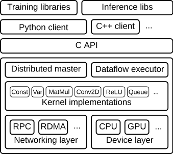{: width="300"} - -**Figure 1** - - -This document focuses on the following layers: - -* **Client**: - * Defines the computation as a dataflow graph. - * Initiates graph execution using a [**session**]( - https://www.tensorflow.org/code/tensorflow/python/client/session.py). -* **Distributed Master** - * Prunes a specific subgraph from the graph, as defined by the arguments - to Session.run(). - * Partitions the subgraph into multiple pieces that run in different - processes and devices. - * Distributes the graph pieces to worker services. - * Initiates graph piece execution by worker services. -* **Worker Services** (one for each task) - * Schedule the execution of graph operations using kernel implementations - appropriate to the available hardware (CPUs, GPUs, etc). - * Send and receive operation results to and from other worker services. -* **Kernel Implementations** - * Perform the computation for individual graph operations. - -Figure 2 illustrates the interaction of these components. "/job:worker/task:0" and -"/job:ps/task:0" are both tasks with worker services. "PS" stands for "parameter -server": a task responsible for storing and updating the model's parameters. -Other tasks send updates to these parameters as they work on optimizing the -parameters. This particular division of labor between tasks is not required, but - is common for distributed training. - -{: width="500"} - -**Figure 2** - -Note that the Distributed Master and Worker Service only exist in -distributed TensorFlow. The single-process version of TensorFlow includes a -special Session implementation that does everything the distributed master does -but only communicates with devices in the local process. - -The following sections describe the core TensorFlow layers in greater detail and -step through the processing of an example graph. - -## Client - -Users write the client TensorFlow program that builds the computation graph. -This program can either directly compose individual operations or use a -convenience library like the Estimators API to compose neural network layers and -other higher-level abstractions. TensorFlow supports multiple client -languages, and we have prioritized Python and C++, because our internal users -are most familiar with these languages. As features become more established, -we typically port them to C++, so that users can access an optimized -implementation from all client languages. Most of the training libraries are -still Python-only, but C++ does have support for efficient inference. - -The client creates a session, which sends the graph definition to the -distributed master as a `tf.GraphDef` -protocol buffer. When the client evaluates a node or nodes in the -graph, the evaluation triggers a call to the distributed master to initiate -computation. - -In Figure 3, the client has built a graph that applies weights (w) to a -feature vector (x), adds a bias term (b) and saves the result in a variable -(s). - -{: width="700"} - -**Figure 3** - -### Code - -* `tf.Session` - -## Distributed master - -The distributed master: - -* prunes the graph to obtain the subgraph required to evaluate the nodes - requested by the client, -* partitions the graph to obtain graph pieces for - each participating device, and -* caches these pieces so that they may be re-used in subsequent steps. - -Since the master sees the overall computation for -a step, it applies standard optimizations such as common subexpression -elimination and constant folding. It then coordinates execution of the -optimized subgraphs across a set of tasks. - -{: width="700"} - -**Figure 4** - - -Figure 5 shows a possible partition of our example graph. The distributed -master has grouped the model parameters in order to place them together on the -parameter server. - -{: width="700"} - -**Figure 5** - - -Where graph edges are cut by the partition, the distributed master inserts -send and receive nodes to pass information between the distributed tasks -(Figure 6). - -{: width="700"} - -**Figure 6** - - -The distributed master then ships the graph pieces to the distributed tasks. - -{: width="700"} - -**Figure 7** - -### Code - -* [MasterService API definition](https://www.tensorflow.org/code/tensorflow/core/protobuf/master_service.proto) -* [Master interface](https://www.tensorflow.org/code/tensorflow/core/distributed_runtime/master_interface.h) - -## Worker Service - -The worker service in each task: - -* handles requests from the master, -* schedules the execution of the kernels for the operations that comprise a - local subgraph, and -* mediates direct communication between tasks. - -We optimize the worker service for running large graphs with low overhead. Our -current implementation can execute tens of thousands of subgraphs per second, -which enables a large number of replicas to make rapid, fine-grained training -steps. The worker service dispatches kernels to local devices and runs kernels -in parallel when possible, for example by using multiple CPU cores or GPU -streams. - -We specialize Send and Recv operations for each pair of source and destination -device types: - -* Transfers between local CPU and GPU devices use the - `cudaMemcpyAsync()` API to overlap computation and data transfer. -* Transfers between two local GPUs use peer-to-peer DMA, to avoid an expensive - copy via the host CPU. - -For transfers between tasks, TensorFlow uses multiple protocols, including: - -* gRPC over TCP. -* RDMA over Converged Ethernet. - -We also have preliminary support for NVIDIA's NCCL library for multi-GPU -communication (see [`tf.contrib.nccl`]( -https://www.tensorflow.org/code/tensorflow/contrib/nccl/python/ops/nccl_ops.py)). - -{: width="700"} - -**Figure 8** - -### Code - -* [WorkerService API definition](https://www.tensorflow.org/code/tensorflow/core/protobuf/worker_service.proto) -* [Worker interface](https://www.tensorflow.org/code/tensorflow/core/distributed_runtime/worker_interface.h) -* [Remote rendezvous (for Send and Recv implementations)](https://www.tensorflow.org/code/tensorflow/core/distributed_runtime/rpc/rpc_rendezvous_mgr.h) - -## Kernel Implementations - -The runtime contains over 200 standard operations including mathematical, array -manipulation, control flow, and state management operations. Each of these -operations can have kernel implementations optimized for a variety of devices. -Many of the operation kernels are implemented using Eigen::Tensor, which uses -C++ templates to generate efficient parallel code for multicore CPUs and GPUs; -however, we liberally use libraries like cuDNN where a more efficient kernel -implementation is possible. We have also implemented -[quantization](../performance/quantization.md), which enables -faster inference in environments such as mobile devices and high-throughput -datacenter applications, and use the -[gemmlowp](https://github.com/google/gemmlowp) low-precision matrix library to -accelerate quantized computation. - -If it is difficult or inefficient to represent a subcomputation as a composition -of operations, users can register additional kernels that provide an efficient -implementation written in C++. For example, we recommend registering your own -fused kernels for some performance critical operations, such as the ReLU and -Sigmoid activation functions and their corresponding gradients. The [XLA Compiler](../performance/xla/index.md) has an -experimental implementation of automatic kernel fusion. - -### Code - -* [`OpKernel` interface](https://www.tensorflow.org/code/tensorflow/core/framework/op_kernel.h) diff --git a/tensorflow/docs_src/extend/index.md b/tensorflow/docs_src/extend/index.md deleted file mode 100644 index bbf4a8139b..0000000000 --- a/tensorflow/docs_src/extend/index.md +++ /dev/null @@ -1,34 +0,0 @@ -# Extend - -This section explains how developers can add functionality to TensorFlow's -capabilities. Begin by reading the following architectural overview: - - * [TensorFlow Architecture](../extend/architecture.md) - -The following guides explain how to extend particular aspects of -TensorFlow: - - * [Adding a New Op](../extend/adding_an_op.md), which explains how to create your own - operations. - * [Adding a Custom Filesystem Plugin](../extend/add_filesys.md), which explains how to - add support for your own shared or distributed filesystem. - * [Custom Data Readers](../extend/new_data_formats.md), which details how to add support - for your own file and record formats. - -Python is currently the only language supported by TensorFlow's API stability -promises. However, TensorFlow also provides functionality in C++, Go, Java and -[JavaScript](https://js.tensorflow.org) (including -[Node.js](https://github.com/tensorflow/tfjs-node)), -plus community support for [Haskell](https://github.com/tensorflow/haskell) and -[Rust](https://github.com/tensorflow/rust). If you'd like to create or -develop TensorFlow features in a language other than these languages, read the -following guide: - - * [TensorFlow in Other Languages](../extend/language_bindings.md) - -To create tools compatible with TensorFlow's model format, read the following -guide: - - * [A Tool Developer's Guide to TensorFlow Model Files](../extend/tool_developers/index.md) - - diff --git a/tensorflow/docs_src/extend/language_bindings.md b/tensorflow/docs_src/extend/language_bindings.md deleted file mode 100644 index 4727eabdc1..0000000000 --- a/tensorflow/docs_src/extend/language_bindings.md +++ /dev/null @@ -1,231 +0,0 @@ -# TensorFlow in other languages - -## Background - -This document is intended as a guide for those interested in the creation or -development of TensorFlow functionality in other programming languages. It -describes the features of TensorFlow and recommended steps for making the same -available in other programming languages. - -Python was the first client language supported by TensorFlow and currently -supports the most features. More and more of that functionality is being moved -into the core of TensorFlow (implemented in C++) and exposed via a [C API]. -Client languages should use the language's [foreign function interface -(FFI)](https://en.wikipedia.org/wiki/Foreign_function_interface) to call into -this [C API] to provide TensorFlow functionality. - -## Overview - -Providing TensorFlow functionality in a programming language can be broken down -into broad categories: - -- *Run a predefined graph*: Given a `GraphDef` (or - `MetaGraphDef`) protocol message, be able to create a session, run queries, - and get tensor results. This is sufficient for a mobile app or server that - wants to run inference on a pre-trained model. -- *Graph construction*: At least one function per defined - TensorFlow op that adds an operation to the graph. Ideally these functions - would be automatically generated so they stay in sync as the op definitions - are modified. -- *Gradients (AKA automatic differentiation)*: Given a graph and a list of - input and output operations, add operations to the graph that compute the - partial derivatives (gradients) of the inputs with respect to the outputs. - Allows for customization of the gradient function for a particular operation - in the graph. -- *Functions*: Define a subgraph that may be called in multiple places in the - main `GraphDef`. Defines a `FunctionDef` in the `FunctionDefLibrary` - included in a `GraphDef`. -- *Control Flow*: Construct "If" and "While" with user-specified subgraphs. - Ideally these work with gradients (see above). -- *Neural Network library*: A number of components that together support the - creation of neural network models and training them (possibly in a - distributed setting). While it would be convenient to have this available in - other languages, there are currently no plans to support this in languages - other than Python. These libraries are typically wrappers over the features - described above. - -At a minimum, a language binding should support running a predefined graph, but -most should also support graph construction. The TensorFlow Python API provides -all these features. - -## Current Status - -New language support should be built on top of the [C API]. However, as you can -see in the table below, not all functionality is available in C yet. Providing -more functionality in the [C API] is an ongoing project. - -Feature | Python | C -:--------------------------------------------- | :---------------------------------------------------------- | :-- -Run a predefined Graph | `tf.import_graph_def`, `tf.Session` | `TF_GraphImportGraphDef`, `TF_NewSession` -Graph construction with generated op functions | Yes | Yes (The C API supports client languages that do this) -Gradients | `tf.gradients` | -Functions | `tf.python.framework.function.Defun` | -Control Flow | `tf.cond`, `tf.while_loop` | -Neural Network library | `tf.train`, `tf.nn`, `tf.contrib.layers`, `tf.contrib.slim` | - -## Recommended Approach - -### Run a predefined graph - -A language binding is expected to define the following classes: - -- `Graph`: A graph representing a TensorFlow computation. Consists of - operations (represented in the client language by `Operation`s) and - corresponds to a `TF_Graph` in the C API. Mainly used as an argument when - creating new `Operation` objects and when starting a `Session`. Also - supports iterating through the operations in the graph - (`TF_GraphNextOperation`), looking up operations by name - (`TF_GraphOperationByName`), and converting to and from a `GraphDef` - protocol message (`TF_GraphToGraphDef` and `TF_GraphImportGraphDef` in the C - API). -- `Operation`: Represents a computation node in the graph. Corresponds to a - `TF_Operation` in the C API. -- `Output`: Represents one of the outputs of an operation in the graph. Has a - `DataType` (and eventually a shape). May be passed as an input argument to a - function for adding operations to a graph, or to a `Session`'s `Run()` - method to fetch that output as a tensor. Corresponds to a `TF_Output` in the - C API. -- `Session`: Represents a client to a particular instance of the TensorFlow - runtime. Its main job is to be constructed with a `Graph` and some options - and then field calls to `Run()` the graph. Corresponds to a `TF_Session` in - the C API. -- `Tensor`: Represents an N-dimensional (rectangular) array with elements all - the same `DataType`. Gets data into and out of a `Session`'s `Run()` call. - Corresponds to a `TF_Tensor` in the C API. -- `DataType`: An enumerant with all the possible tensor types supported by - TensorFlow. Corresponds to `TF_DataType` in the C API and often referred to - as `dtype` in the Python API. - -### Graph construction - -TensorFlow has many ops, and the list is not static, so we recommend generating -the functions for adding ops to a graph instead of writing them by individually -by hand (though writing a few by hand is a good way to figure out what the -generator should generate). The information needed to generate a function is -contained in an `OpDef` protocol message. - -There are a few ways to get a list of the `OpDef`s for the registered ops: - -- `TF_GetAllOpList` in the C API retrieves all registered `OpDef` protocol - messages. This can be used to write the generator in the client language. - This requires that the client language have protocol buffer support in order - to interpret the `OpDef` messages. -- The C++ function `OpRegistry::Global()->GetRegisteredOps()` returns the same - list of all registered `OpDef`s (defined in - [`tensorflow/core/framework/op.h`](https://www.tensorflow.org/code/tensorflow/core/framework/op.h)). This can be used to write the generator - in C++ (particularly useful for languages that do not have protocol buffer - support). -- The ASCII-serialized version of that list is periodically checked in to - [`tensorflow/core/ops/ops.pbtxt`](https://www.tensorflow.org/code/tensorflow/core/ops/ops.pbtxt) by an automated process. - -The `OpDef` specifies the following: - -- Name of the op in CamelCase. For generated functions follow the conventions - of the language. For example, if the language uses snake_case, use that - instead of CamelCase for the op's function name. -- A list of inputs and outputs. The types for these may be polymorphic by - referencing attributes, as described in the inputs and outputs section of - [Adding an op](../extend/adding_an_op.md). -- A list of attributes, along with their default values (if any). Note that - some of these will be inferred (if they are determined by an input), some - will be optional (if they have a default), and some will be required (no - default). -- Documentation for the op in general and the inputs, outputs, and - non-inferred attributes. -- Some other fields that are used by the runtime and can be ignored by the - code generators. - -An `OpDef` can be converted into the text of a function that adds that op to the -graph using the `TF_OperationDescription` C API (wrapped in the language's FFI): - -- Start with `TF_NewOperation()` to create the `TF_OperationDescription*`. -- Call `TF_AddInput()` or `TF_AddInputList()` once per input (depending on - whether the input has a list type). -- Call `TF_SetAttr*()` functions to set non-inferred attributes. May skip - attributes with defaults if you don't want to override the default value. -- Set optional fields if necessary: - - `TF_SetDevice()`: force the operation onto a specific device. - - `TF_AddControlInput()`: add requirements that another operation finish - before this operation starts running - - `TF_SetAttrString("_kernel")` to set the kernel label (rarely used) - - `TF_ColocateWith()` to colocate one op with another -- Call `TF_FinishOperation()` when done. This adds the operation to the graph, - after which it can't be modified. - -The existing examples run the code generator as part of the build process (using -a Bazel genrule). Alternatively, the code generator can be run by an automated -cron process, possibly checking in the result. This creates a risk of divergence -between the generated code and the `OpDef`s checked into the repository, but is -useful for languages where code is expected to be generated ahead of time like -`go get` for Go and `cargo ops` for Rust. At the other end of the spectrum, for -some languages the code could be generated dynamically from -[`tensorflow/core/ops/ops.pbtxt`](https://www.tensorflow.org/code/tensorflow/core/ops/ops.pbtxt). - -#### Handling Constants - -Calling code will be much more concise if users can provide constants to input -arguments. The generated code should convert those constants to operations that -are added to the graph and used as input to the op being instantiated. - -#### Optional parameters - -If the language allows for optional parameters to a function (like keyword -arguments with defaults in Python), use them for optional attributes, operation -names, devices, control inputs etc. In some languages, these optional parameters -can be set using dynamic scopes (like "with" blocks in Python). Without these -features, the library may resort to the "builder pattern", as is done in the C++ -version of the TensorFlow API. - -#### Name scopes - -It is a good idea to have support for naming graph operations using some sort of -scoping hierarchy, especially considering the fact that TensorBoard relies on it -to display large graphs in a reasonable way. The existing Python and C++ APIs -take different approaches: In Python, the "directory" part of the name -(everything up to the last "/") comes from `with` blocks. In effect, there is a -thread-local stack with the scopes defining the name hierarchy. The last -component of the name is either supplied explicitly by the user (using the -optional `name` keyword argument) or defaults to the name of the type of the op -being added. In C++ the "directory" part of the name is stored in an explicit -`Scope` object. The `NewSubScope()` method appends to that part of the name and -returns a new `Scope`. The last component of the name is set using the -`WithOpName()` method, and like Python defaults to the name of the type of op -being added. `Scope` objects are explicitly passed around to specify the name of -the context. - -#### Wrappers - -It may make sense to keep the generated functions private for some ops so that -wrapper functions that do a little bit of additional work can be used instead. -This also gives an escape hatch for supporting features outside the scope of -generated code. - -One use of a wrapper is for supporting `SparseTensor` input and output. A -`SparseTensor` is a tuple of 3 dense tensors: indices, values, and shape. values -is a vector size [n], shape is a vector size [rank], and indices is a matrix -size [n, rank]. There are some sparse ops that use this triple to represent a -single sparse tensor. - -Another reason to use wrappers is for ops that hold state. There are a few such -ops (e.g. a variable) that have several companion ops for operating on that -state. The Python API has classes for these ops where the constructor creates -the op, and methods on that class add operations to the graph that operate on -the state. - -#### Other Considerations - -- It is good to have a list of keywords used to rename op functions and - arguments that collide with language keywords (or other symbols that will - cause trouble, like the names of library functions or variables referenced - in the generated code). -- The function for adding a `Const` operation to a graph typically is a - wrapper since the generated function will typically have redundant - `DataType` inputs. - -### Gradients, functions and control flow - -At this time, support for gradients, functions and control flow operations ("if" -and "while") is not available in languages other than Python. This will be -updated when the [C API] provides necessary support. - -[C API]: https://www.tensorflow.org/code/tensorflow/c/c_api.h diff --git a/tensorflow/docs_src/extend/leftnav_files b/tensorflow/docs_src/extend/leftnav_files deleted file mode 100644 index 12315b711b..0000000000 --- a/tensorflow/docs_src/extend/leftnav_files +++ /dev/null @@ -1,7 +0,0 @@ -index.md -architecture.md -adding_an_op.md -add_filesys.md -new_data_formats.md -language_bindings.md -tool_developers/index.md diff --git a/tensorflow/docs_src/extend/new_data_formats.md b/tensorflow/docs_src/extend/new_data_formats.md deleted file mode 100644 index 7ca50c9c76..0000000000 --- a/tensorflow/docs_src/extend/new_data_formats.md +++ /dev/null @@ -1,305 +0,0 @@ -# Reading custom file and record formats - -PREREQUISITES: - -* Some familiarity with C++. -* Must have - [downloaded TensorFlow source](../install/install_sources.md), and be - able to build it. - -We divide the task of supporting a file format into two pieces: - -* File formats: We use a reader `tf.data.Dataset` to read raw *records* (which - are typically represented by scalar string tensors, but can have more - structure) from a file. -* Record formats: We use decoder or parsing ops to turn a string record - into tensors usable by TensorFlow. - -For example, to re-implement `tf.contrib.data.make_csv_dataset` function, we -could use `tf.data.TextLineDataset` to extract the records, and then -use `tf.data.Dataset.map` and `tf.decode_csv` to parses the CSV records from -each line of text in the dataset. - -[TOC] - -## Writing a `Dataset` for a file format - -A `tf.data.Dataset` represents a sequence of *elements*, which can be the -individual records in a file. There are several examples of "reader" datasets -that are already built into TensorFlow: - -* `tf.data.TFRecordDataset` - ([source in `kernels/data/reader_dataset_ops.cc`](https://www.tensorflow.org/code/tensorflow/core/kernels/data/reader_dataset_ops.cc)) -* `tf.data.FixedLengthRecordDataset` - ([source in `kernels/data/reader_dataset_ops.cc`](https://www.tensorflow.org/code/tensorflow/core/kernels/data/reader_dataset_ops.cc)) -* `tf.data.TextLineDataset` - ([source in `kernels/data/reader_dataset_ops.cc`](https://www.tensorflow.org/code/tensorflow/core/kernels/data/reader_dataset_ops.cc)) - -Each of these implementations comprises three related classes: - -* A `tensorflow::DatasetOpKernel` subclass (e.g. `TextLineDatasetOp`), which - tells TensorFlow how to construct a dataset object from the inputs to and - attrs of an op, in its `MakeDataset()` method. - -* A `tensorflow::GraphDatasetBase` subclass (e.g. `TextLineDatasetOp::Dataset`), - which represents the *immutable* definition of the dataset itself, and tells - TensorFlow how to construct an iterator object over that dataset, in its - `MakeIteratorInternal()` method. - -* A `tensorflow::DatasetIterator<Dataset>` subclass (e.g. - `TextLineDatasetOp::Dataset::Iterator`), which represents the *mutable* state - of an iterator over a particular dataset, and tells TensorFlow how to get the - next element from the iterator, in its `GetNextInternal()` method. - -The most important method is the `GetNextInternal()` method, since it defines -how to actually read records from the file and represent them as one or more -`Tensor` objects. - -To create a new reader dataset called (for example) `MyReaderDataset`, you will -need to: - -1. In C++, define subclasses of `tensorflow::DatasetOpKernel`, - `tensorflow::GraphDatasetBase`, and `tensorflow::DatasetIterator<Dataset>` - that implement the reading logic. -2. In C++, register a new reader op and kernel with the name - `"MyReaderDataset"`. -3. In Python, define a subclass of `tf.data.Dataset` called `MyReaderDataset`. - -You can put all the C++ code in a single file, such as -`my_reader_dataset_op.cc`. It will help if you are -familiar with [the adding an op how-to](../extend/adding_an_op.md). The following skeleton -can be used as a starting point for your implementation: - -```c++ -#include "tensorflow/core/framework/common_shape_fns.h" -#include "tensorflow/core/framework/dataset.h" -#include "tensorflow/core/framework/op.h" -#include "tensorflow/core/framework/shape_inference.h" - -namespace myproject { -namespace { - -using ::tensorflow::DT_STRING; -using ::tensorflow::PartialTensorShape; -using ::tensorflow::Status; - -class MyReaderDatasetOp : public tensorflow::DatasetOpKernel { - public: - - MyReaderDatasetOp(tensorflow::OpKernelConstruction* ctx) - : DatasetOpKernel(ctx) { - // Parse and validate any attrs that define the dataset using - // `ctx->GetAttr()`, and store them in member variables. - } - - void MakeDataset(tensorflow::OpKernelContext* ctx, - tensorflow::DatasetBase** output) override { - // Parse and validate any input tensors 0that define the dataset using - // `ctx->input()` or the utility function - // `ParseScalarArgument<T>(ctx, &arg)`. - - // Create the dataset object, passing any (already-validated) arguments from - // attrs or input tensors. - *output = new Dataset(ctx); - } - - private: - class Dataset : public tensorflow::GraphDatasetBase { - public: - Dataset(tensorflow::OpKernelContext* ctx) : GraphDatasetBase(ctx) {} - - std::unique_ptr<tensorflow::IteratorBase> MakeIteratorInternal( - const string& prefix) const override { - return std::unique_ptr<tensorflow::IteratorBase>(new Iterator( - {this, tensorflow::strings::StrCat(prefix, "::MyReader")})); - } - - // Record structure: Each record is represented by a scalar string tensor. - // - // Dataset elements can have a fixed number of components of different - // types and shapes; replace the following two methods to customize this - // aspect of the dataset. - const tensorflow::DataTypeVector& output_dtypes() const override { - static auto* const dtypes = new tensorflow::DataTypeVector({DT_STRING}); - return *dtypes; - } - const std::vector<PartialTensorShape>& output_shapes() const override { - static std::vector<PartialTensorShape>* shapes = - new std::vector<PartialTensorShape>({{}}); - return *shapes; - } - - string DebugString() const override { return "MyReaderDatasetOp::Dataset"; } - - protected: - // Optional: Implementation of `GraphDef` serialization for this dataset. - // - // Implement this method if you want to be able to save and restore - // instances of this dataset (and any iterators over it). - Status AsGraphDefInternal(DatasetGraphDefBuilder* b, - tensorflow::Node** output) const override { - // Construct nodes to represent any of the input tensors from this - // object's member variables using `b->AddScalar()` and `b->AddVector()`. - std::vector<tensorflow::Node*> input_tensors; - TF_RETURN_IF_ERROR(b->AddDataset(this, input_tensors, output)); - return Status::OK(); - } - - private: - class Iterator : public tensorflow::DatasetIterator<Dataset> { - public: - explicit Iterator(const Params& params) - : DatasetIterator<Dataset>(params), i_(0) {} - - // Implementation of the reading logic. - // - // The example implementation in this file yields the string "MyReader!" - // ten times. In general there are three cases: - // - // 1. If an element is successfully read, store it as one or more tensors - // in `*out_tensors`, set `*end_of_sequence = false` and return - // `Status::OK()`. - // 2. If the end of input is reached, set `*end_of_sequence = true` and - // return `Status::OK()`. - // 3. If an error occurs, return an error status using one of the helper - // functions from "tensorflow/core/lib/core/errors.h". - Status GetNextInternal(tensorflow::IteratorContext* ctx, - std::vector<tensorflow::Tensor>* out_tensors, - bool* end_of_sequence) override { - // NOTE: `GetNextInternal()` may be called concurrently, so it is - // recommended that you protect the iterator state with a mutex. - tensorflow::mutex_lock l(mu_); - if (i_ < 10) { - // Create a scalar string tensor and add it to the output. - tensorflow::Tensor record_tensor(ctx->allocator({}), DT_STRING, {}); - record_tensor.scalar<string>()() = "MyReader!"; - out_tensors->emplace_back(std::move(record_tensor)); - ++i_; - *end_of_sequence = false; - } else { - *end_of_sequence = true; - } - return Status::OK(); - } - - protected: - // Optional: Implementation of iterator state serialization for this - // iterator. - // - // Implement these two methods if you want to be able to save and restore - // instances of this iterator. - Status SaveInternal(tensorflow::IteratorStateWriter* writer) override { - tensorflow::mutex_lock l(mu_); - TF_RETURN_IF_ERROR(writer->WriteScalar(full_name("i"), i_)); - return Status::OK(); - } - Status RestoreInternal(tensorflow::IteratorContext* ctx, - tensorflow::IteratorStateReader* reader) override { - tensorflow::mutex_lock l(mu_); - TF_RETURN_IF_ERROR(reader->ReadScalar(full_name("i"), &i_)); - return Status::OK(); - } - - private: - tensorflow::mutex mu_; - int64 i_ GUARDED_BY(mu_); - }; - }; -}; - -// Register the op definition for MyReaderDataset. -// -// Dataset ops always have a single output, of type `variant`, which represents -// the constructed `Dataset` object. -// -// Add any attrs and input tensors that define the dataset here. -REGISTER_OP("MyReaderDataset") - .Output("handle: variant") - .SetIsStateful() - .SetShapeFn(tensorflow::shape_inference::ScalarShape); - -// Register the kernel implementation for MyReaderDataset. -REGISTER_KERNEL_BUILDER(Name("MyReaderDataset").Device(tensorflow::DEVICE_CPU), - MyReaderDatasetOp); - -} // namespace -} // namespace myproject -``` - -The last step is to build the C++ code and add a Python wrapper. The easiest way -to do this is by [compiling a dynamic -library](../extend/adding_an_op.md#build_the_op_library) (e.g. called `"my_reader_dataset_op.so"`), and adding a Python class -that subclasses `tf.data.Dataset` to wrap it. An example Python program is -given here: - -```python -import tensorflow as tf - -# Assumes the file is in the current working directory. -my_reader_dataset_module = tf.load_op_library("./my_reader_dataset_op.so") - -class MyReaderDataset(tf.data.Dataset): - - def __init__(self): - super(MyReaderDataset, self).__init__() - # Create any input attrs or tensors as members of this class. - - def _as_variant_tensor(self): - # Actually construct the graph node for the dataset op. - # - # This method will be invoked when you create an iterator on this dataset - # or a dataset derived from it. - return my_reader_dataset_module.my_reader_dataset() - - # The following properties define the structure of each element: a scalar - # `tf.string` tensor. Change these properties to match the `output_dtypes()` - # and `output_shapes()` methods of `MyReaderDataset::Dataset` if you modify - # the structure of each element. - @property - def output_types(self): - return tf.string - - @property - def output_shapes(self): - return tf.TensorShape([]) - - @property - def output_classes(self): - return tf.Tensor - -if __name__ == "__main__": - # Create a MyReaderDataset and print its elements. - with tf.Session() as sess: - iterator = MyReaderDataset().make_one_shot_iterator() - next_element = iterator.get_next() - try: - while True: - print(sess.run(next_element)) # Prints "MyReader!" ten times. - except tf.errors.OutOfRangeError: - pass -``` - -You can see some examples of `Dataset` wrapper classes in -[`tensorflow/python/data/ops/dataset_ops.py`](https://www.tensorflow.org/code/tensorflow/python/data/ops/dataset_ops.py). - -## Writing an Op for a record format - -Generally this is an ordinary op that takes a scalar string record as input, and -so follow [the instructions to add an Op](../extend/adding_an_op.md). -You may optionally take a scalar string key as input, and include that in error -messages reporting improperly formatted data. That way users can more easily -track down where the bad data came from. - -Examples of Ops useful for decoding records: - -* `tf.parse_single_example` (and `tf.parse_example`) -* `tf.decode_csv` -* `tf.decode_raw` - -Note that it can be useful to use multiple Ops to decode a particular record -format. For example, you may have an image saved as a string in -[a `tf.train.Example` protocol buffer](https://www.tensorflow.org/code/tensorflow/core/example/example.proto). -Depending on the format of that image, you might take the corresponding output -from a `tf.parse_single_example` op and call `tf.image.decode_jpeg`, -`tf.image.decode_png`, or `tf.decode_raw`. It is common to take the output -of `tf.decode_raw` and use `tf.slice` and `tf.reshape` to extract pieces. diff --git a/tensorflow/docs_src/extend/tool_developers/index.md b/tensorflow/docs_src/extend/tool_developers/index.md deleted file mode 100644 index f02cd23be8..0000000000 --- a/tensorflow/docs_src/extend/tool_developers/index.md +++ /dev/null @@ -1,186 +0,0 @@ -# A Tool Developer's Guide to TensorFlow Model Files - -Most users shouldn't need to care about the internal details of how TensorFlow -stores data on disk, but you might if you're a tool developer. For example, you -may want to analyze models, or convert back and forth between TensorFlow and -other formats. This guide tries to explain some of the details of how you can -work with the main files that hold model data, to make it easier to develop -those kind of tools. - -[TOC] - -## Protocol Buffers - -All of TensorFlow's file formats are based on -[Protocol Buffers](https://developers.google.com/protocol-buffers/?hl=en), so to -start it's worth getting familiar with how they work. The summary is that you -define data structures in text files, and the protobuf tools generate classes in -C, Python, and other languages that can load, save, and access the data in a -friendly way. We often refer to Protocol Buffers as protobufs, and I'll use -that convention in this guide. - -## GraphDef - -The foundation of computation in TensorFlow is the `Graph` object. This holds a -network of nodes, each representing one operation, connected to each other as -inputs and outputs. After you've created a `Graph` object, you can save it out -by calling `as_graph_def()`, which returns a `GraphDef` object. - -The GraphDef class is an object created by the ProtoBuf library from the -definition in -[tensorflow/core/framework/graph.proto](https://github.com/tensorflow/tensorflow/blob/master/tensorflow/core/framework/graph.proto). The protobuf tools parse -this text file, and generate the code to load, store, and manipulate graph -definitions. If you see a standalone TensorFlow file representing a model, it's -likely to contain a serialized version of one of these `GraphDef` objects -saved out by the protobuf code. - -This generated code is used to save and load the GraphDef files from disk. The code that actually loads the model looks like this: - -```python -graph_def = graph_pb2.GraphDef() -``` - -This line creates an empty `GraphDef` object, the class that's been created -from the textual definition in graph.proto. This is the object we're going to -populate with the data from our file. - -```python -with open(FLAGS.graph, "rb") as f: -``` - -Here we get a file handle for the path we've passed in to the script - -```python - if FLAGS.input_binary: - graph_def.ParseFromString(f.read()) - else: - text_format.Merge(f.read(), graph_def) -``` - -## Text or Binary? - -There are actually two different formats that a ProtoBuf can be saved in. -TextFormat is a human-readable form, which makes it nice for debugging and -editing, but can get large when there's numerical data like weights stored in -it. You can see a small example of that in -[graph_run_run2.pbtxt](https://github.com/tensorflow/tensorboard/blob/master/tensorboard/demo/data/graph_run_run2.pbtxt). - -Binary format files are a lot smaller than their text equivalents, even though -they're not as readable for us. In this script, we ask the user to supply a -flag indicating whether the input file is binary or text, so we know the right -function to call. You can find an example of a large binary file inside the -[inception_v3 archive](https://storage.googleapis.com/download.tensorflow.org/models/inception_v3_2016_08_28_frozen.pb.tar.gz), -as `inception_v3_2016_08_28_frozen.pb`. - -The API itself can be a bit confusing - the binary call is actually -`ParseFromString()`, whereas you use a utility function from the `text_format` -module to load textual files. - -## Nodes - -Once you've loaded a file into the `graph_def` variable, you can now access the -data inside it. For most practical purposes, the important section is the list -of nodes stored in the node member. Here's the code that loops through those: - -```python -for node in graph_def.node -``` - -Each node is a `NodeDef` object, defined in -[tensorflow/core/framework/node_def.proto](https://github.com/tensorflow/tensorflow/blob/master/tensorflow/core/framework/node_def.proto). These -are the fundamental building blocks of TensorFlow graphs, with each one defining -a single operation along with its input connections. Here are the members of a -`NodeDef`, and what they mean. - -### `name` - -Every node should have a unique identifier that's not used by any other nodes -in the graph. If you don't specify one as you're building a graph using the -Python API, one reflecting the name of operation, such as "MatMul", -concatenated with a monotonically increasing number, such as "5", will be -picked for you. The name is used when defining the connections between nodes, -and when setting inputs and outputs for the whole graph when it's run. - -### `op` - -This defines what operation to run, for example `"Add"`, `"MatMul"`, or -`"Conv2D"`. When a graph is run, this op name is looked up in a registry to -find an implementation. The registry is populated by calls to the -`REGISTER_OP()` macro, like those in -[tensorflow/core/ops/nn_ops.cc](https://github.com/tensorflow/tensorflow/blob/master/tensorflow/core/ops/nn_ops.cc). - -### `input` - -A list of strings, each one of which is the name of another node, optionally -followed by a colon and an output port number. For example, a node with two -inputs might have a list like `["some_node_name", "another_node_name"]`, which -is equivalent to `["some_node_name:0", "another_node_name:0"]`, and defines the -node's first input as the first output from the node with the name -`"some_node_name"`, and a second input from the first output of -`"another_node_name"` - -### `device` - -In most cases you can ignore this, since it defines where to run a node in a -distributed environment, or when you want to force the operation onto CPU or -GPU. - -### `attr` - -This is a key/value store holding all the attributes of a node. These are the -permanent properties of nodes, things that don't change at runtime such as the -size of filters for convolutions, or the values of constant ops. Because there -can be so many different types of attribute values, from strings, to ints, to -arrays of tensor values, there's a separate protobuf file defining the data -structure that holds them, in -[tensorflow/core/framework/attr_value.proto](https://github.com/tensorflow/tensorflow/blob/master/tensorflow/core/framework/attr_value.proto). - -Each attribute has a unique name string, and the expected attributes are listed -when the operation is defined. If an attribute isn't present in a node, but it -has a default listed in the operation definition, that default is used when the -graph is created. - -You can access all of these members by calling `node.name`, `node.op`, etc. in -Python. The list of nodes stored in the `GraphDef` is a full definition of the -model architecture. - -## Freezing - -One confusing part about this is that the weights usually aren't stored inside -the file format during training. Instead, they're held in separate checkpoint -files, and there are `Variable` ops in the graph that load the latest values -when they're initialized. It's often not very convenient to have separate files -when you're deploying to production, so there's the -[freeze_graph.py](https://github.com/tensorflow/tensorflow/blob/master/tensorflow/python/tools/freeze_graph.py) script that takes a graph definition and a set -of checkpoints and freezes them together into a single file. - -What this does is load the `GraphDef`, pull in the values for all the variables -from the latest checkpoint file, and then replace each `Variable` op with a -`Const` that has the numerical data for the weights stored in its attributes -It then strips away all the extraneous nodes that aren't used for forward -inference, and saves out the resulting `GraphDef` into an output file. - -## Weight Formats - -If you're dealing with TensorFlow models that represent neural networks, one of -the most common problems is extracting and interpreting the weight values. A -common way to store them, for example in graphs created by the freeze_graph -script, is as `Const` ops containing the weights as `Tensors`. These are -defined in -[tensorflow/core/framework/tensor.proto](https://github.com/tensorflow/tensorflow/blob/master/tensorflow/core/framework/tensor.proto), and contain information -about the size and type of the data, as well as the values themselves. In -Python, you get a `TensorProto` object from a `NodeDef` representing a `Const` -op by calling something like `some_node_def.attr['value'].tensor`. - -This will give you an object representing the weights data. The data itself -will be stored in one of the lists with the suffix _val as indicated by the -type of the object, for example `float_val` for 32-bit float data types. - -The ordering of convolution weight values is often tricky to deal with when -converting between different frameworks. In TensorFlow, the filter weights for -the `Conv2D` operation are stored on the second input, and are expected to be -in the order `[filter_height, filter_width, input_depth, output_depth]`, where -filter_count increasing by one means moving to an adjacent value in memory. - -Hopefully this rundown gives you a better idea of what's going on inside -TensorFlow model files, and will help you if you ever need to manipulate them. diff --git a/tensorflow/docs_src/extras/README.txt b/tensorflow/docs_src/extras/README.txt deleted file mode 100644 index 765809a762..0000000000 --- a/tensorflow/docs_src/extras/README.txt +++ /dev/null @@ -1,3 +0,0 @@ -This directory holds extra files we'd like to be able -to link to and serve from within tensorflow.org. -They are excluded from versioning.
\ No newline at end of file diff --git a/tensorflow/docs_src/guide/autograph.md b/tensorflow/docs_src/guide/autograph.md deleted file mode 100644 index 823e1c6d6b..0000000000 --- a/tensorflow/docs_src/guide/autograph.md +++ /dev/null @@ -1,3 +0,0 @@ -# AutoGraph: Easy control flow for graphs - -[Colab notebook](https://colab.research.google.com/github/tensorflow/models/blob/master/samples/core/guide/autograph.ipynb) diff --git a/tensorflow/docs_src/guide/checkpoints.md b/tensorflow/docs_src/guide/checkpoints.md deleted file mode 100644 index 3c92cbbd40..0000000000 --- a/tensorflow/docs_src/guide/checkpoints.md +++ /dev/null @@ -1,238 +0,0 @@ -# Checkpoints - -This document examines how to save and restore TensorFlow models built with -Estimators. TensorFlow provides two model formats: - -* checkpoints, which is a format dependent on the code that created - the model. -* SavedModel, which is a format independent of the code that created - the model. - -This document focuses on checkpoints. For details on `SavedModel`, see the -[Saving and Restoring](../guide/saved_model.md) guide. - - -## Sample code - -This document relies on the same -[Iris classification example](https://github.com/tensorflow/models/blob/master/samples/core/get_started/premade_estimator.py) detailed in [Getting Started with TensorFlow](../guide/premade_estimators.md). -To download and access the example, invoke the following two commands: - -```shell -git clone https://github.com/tensorflow/models/ -cd models/samples/core/get_started -``` - -Most of the code snippets in this document are minor variations -on `premade_estimator.py`. - - -## Saving partially-trained models - -Estimators automatically write the following to disk: - -* **checkpoints**, which are versions of the model created during training. -* **event files**, which contain information that - [TensorBoard](https://developers.google.com/machine-learning/glossary/#TensorBoard) - uses to create visualizations. - -To specify the top-level directory in which the Estimator stores its -information, assign a value to the optional `model_dir` argument of *any* -`Estimator`'s constructor. -Taking `DNNClassifier` as an example, -the following code sets the `model_dir` -argument to the `models/iris` directory: - -```python -classifier = tf.estimator.DNNClassifier( - feature_columns=my_feature_columns, - hidden_units=[10, 10], - n_classes=3, - model_dir='models/iris') -``` - -Suppose you call the Estimator's `train` method. For example: - - -```python -classifier.train( - input_fn=lambda:train_input_fn(train_x, train_y, batch_size=100), - steps=200) -``` - -As suggested by the following diagrams, the first call to `train` -adds checkpoints and other files to the `model_dir` directory: - -<div style="width:80%; margin:auto; margin-bottom:10px; margin-top:20px;"> -<img style="width:100%" src="../images/first_train_calls.png"> -</div> -<div style="text-align: center"> -The first call to train(). -</div> - - -To see the objects in the created `model_dir` directory on a -UNIX-based system, just call `ls` as follows: - -```none -$ ls -1 models/iris -checkpoint -events.out.tfevents.timestamp.hostname -graph.pbtxt -model.ckpt-1.data-00000-of-00001 -model.ckpt-1.index -model.ckpt-1.meta -model.ckpt-200.data-00000-of-00001 -model.ckpt-200.index -model.ckpt-200.meta -``` - -The preceding `ls` command shows that the Estimator created checkpoints -at steps 1 (the start of training) and 200 (the end of training). - - -### Default checkpoint directory - -If you don't specify `model_dir` in an Estimator's constructor, the Estimator -writes checkpoint files to a temporary directory chosen by Python's -[tempfile.mkdtemp](https://docs.python.org/3/library/tempfile.html#tempfile.mkdtemp) -function. For example, the following Estimator constructor does *not* specify -the `model_dir` argument: - -```python -classifier = tf.estimator.DNNClassifier( - feature_columns=my_feature_columns, - hidden_units=[10, 10], - n_classes=3) - -print(classifier.model_dir) -``` - -The `tempfile.mkdtemp` function picks a secure, temporary directory -appropriate for your operating system. For example, a typical temporary -directory on macOS might be something like the following: - -```None -/var/folders/0s/5q9kfzfj3gx2knj0vj8p68yc00dhcr/T/tmpYm1Rwa -``` - -### Checkpointing Frequency - -By default, the Estimator saves -[checkpoints](https://developers.google.com/machine-learning/glossary/#checkpoint) -in the `model_dir` according to the following schedule: - -* Writes a checkpoint every 10 minutes (600 seconds). -* Writes a checkpoint when the `train` method starts (first iteration) - and completes (final iteration). -* Retains only the 5 most recent checkpoints in the directory. - -You may alter the default schedule by taking the following steps: - -1. Create a `tf.estimator.RunConfig` object that defines the - desired schedule. -2. When instantiating the Estimator, pass that `RunConfig` object to the - Estimator's `config` argument. - -For example, the following code changes the checkpointing schedule to every -20 minutes and retains the 10 most recent checkpoints: - -```python -my_checkpointing_config = tf.estimator.RunConfig( - save_checkpoints_secs = 20*60, # Save checkpoints every 20 minutes. - keep_checkpoint_max = 10, # Retain the 10 most recent checkpoints. -) - -classifier = tf.estimator.DNNClassifier( - feature_columns=my_feature_columns, - hidden_units=[10, 10], - n_classes=3, - model_dir='models/iris', - config=my_checkpointing_config) -``` - -## Restoring your model - -The first time you call an Estimator's `train` method, TensorFlow saves a -checkpoint to the `model_dir`. Each subsequent call to the Estimator's -`train`, `evaluate`, or `predict` method causes the following: - -1. The Estimator builds the model's - [graph](https://developers.google.com/machine-learning/glossary/#graph) - by running the `model_fn()`. (For details on the `model_fn()`, see - [Creating Custom Estimators.](../guide/custom_estimators.md)) -2. The Estimator initializes the weights of the new model from the data - stored in the most recent checkpoint. - -In other words, as the following illustration suggests, once checkpoints -exist, TensorFlow rebuilds the model each time you call `train()`, -`evaluate()`, or `predict()`. - -<div style="width:80%; margin:auto; margin-bottom:10px; margin-top:20px;"> -<img style="width:100%" src="../images/subsequent_calls.png"> -</div> -<div style="text-align: center"> -Subsequent calls to train(), evaluate(), or predict() -</div> - - -### Avoiding a bad restoration - -Restoring a model's state from a checkpoint only works if the model -and checkpoint are compatible. For example, suppose you trained a -`DNNClassifier` Estimator containing two hidden layers, -each having 10 nodes: - -```python -classifier = tf.estimator.DNNClassifier( - feature_columns=feature_columns, - hidden_units=[10, 10], - n_classes=3, - model_dir='models/iris') - -classifier.train( - input_fn=lambda:train_input_fn(train_x, train_y, batch_size=100), - steps=200) -``` - -After training (and, therefore, after creating checkpoints in `models/iris`), -imagine that you changed the number of neurons in each hidden layer from 10 to -20 and then attempted to retrain the model: - -``` python -classifier2 = tf.estimator.DNNClassifier( - feature_columns=my_feature_columns, - hidden_units=[20, 20], # Change the number of neurons in the model. - n_classes=3, - model_dir='models/iris') - -classifier.train( - input_fn=lambda:train_input_fn(train_x, train_y, batch_size=100), - steps=200) -``` - -Since the state in the checkpoint is incompatible with the model described -in `classifier2`, retraining fails with the following error: - -```None -... -InvalidArgumentError (see above for traceback): tensor_name = -dnn/hiddenlayer_1/bias/t_0/Adagrad; shape in shape_and_slice spec [10] -does not match the shape stored in checkpoint: [20] -``` - -To run experiments in which you train and compare slightly different -versions of a model, save a copy of the code that created each -`model_dir`, possibly by creating a separate git branch for each version. -This separation will keep your checkpoints recoverable. - -## Summary - -Checkpoints provide an easy automatic mechanism for saving and restoring -models created by Estimators. - -See the [Saving and Restoring](../guide/saved_model.md) guide for details about: - -* Saving and restoring models using low-level TensorFlow APIs. -* Exporting and importing models in the SavedModel format, which is a - language-neutral, recoverable, serialization format. diff --git a/tensorflow/docs_src/guide/custom_estimators.md b/tensorflow/docs_src/guide/custom_estimators.md deleted file mode 100644 index 913a35920f..0000000000 --- a/tensorflow/docs_src/guide/custom_estimators.md +++ /dev/null @@ -1,602 +0,0 @@ - -# Creating Custom Estimators - -This document introduces custom Estimators. In particular, this document -demonstrates how to create a custom `tf.estimator.Estimator` that -mimics the behavior of the pre-made Estimator -`tf.estimator.DNNClassifier` in solving the Iris problem. See -the [Pre-Made Estimators chapter](../guide/premade_estimators.md) for details -on the Iris problem. - -To download and access the example code invoke the following two commands: - -```shell -git clone https://github.com/tensorflow/models/ -cd models/samples/core/get_started -``` - -In this document we will be looking at -[`custom_estimator.py`](https://github.com/tensorflow/models/blob/master/samples/core/get_started/custom_estimator.py). -You can run it with the following command: - -```bsh -python custom_estimator.py -``` - -If you are feeling impatient, feel free to compare and contrast -[`custom_estimator.py`](https://github.com/tensorflow/models/blob/master/samples/core/get_started/custom_estimator.py) -with -[`premade_estimator.py`](https://github.com/tensorflow/models/blob/master/samples/core/get_started/premade_estimator.py). -(which is in the same directory). - - - -## Pre-made vs. custom - -As the following figure shows, pre-made Estimators are subclasses of the -`tf.estimator.Estimator` base class, while custom Estimators are an instance -of tf.estimator.Estimator: - -<div style="width:100%; margin:auto; margin-bottom:10px; margin-top:20px;"> -<img style="display:block; margin: 0 auto" - alt="Premade estimators are sub-classes of `Estimator`. Custom Estimators are usually (direct) instances of `Estimator`" - src="../images/custom_estimators/estimator_types.png"> -</div> -<div style="text-align: center"> -Pre-made and custom Estimators are all Estimators. -</div> - -Pre-made Estimators are fully baked. Sometimes though, you need more control -over an Estimator's behavior. That's where custom Estimators come in. You can -create a custom Estimator to do just about anything. If you want hidden layers -connected in some unusual fashion, write a custom Estimator. If you want to -calculate a unique -[metric](https://developers.google.com/machine-learning/glossary/#metric) -for your model, write a custom Estimator. Basically, if you want an Estimator -optimized for your specific problem, write a custom Estimator. - -A model function (or `model_fn`) implements the ML algorithm. The -only difference between working with pre-made Estimators and custom Estimators -is: - -* With pre-made Estimators, someone already wrote the model function for you. -* With custom Estimators, you must write the model function. - -Your model function could implement a wide range of algorithms, defining all -sorts of hidden layers and metrics. Like input functions, all model functions -must accept a standard group of input parameters and return a standard group of -output values. Just as input functions can leverage the Dataset API, model -functions can leverage the Layers API and the Metrics API. - -Let's see how to solve the Iris problem with a custom Estimator. A quick -reminder--here's the organization of the Iris model that we're trying to mimic: - -<div style="width:100%; margin:auto; margin-bottom:10px; margin-top:20px;"> -<img style="display:block; margin: 0 auto" - alt="A diagram of the network architecture: Inputs, 2 hidden layers, and outputs" - src="../images/custom_estimators/full_network.png"> -</div> -<div style="text-align: center"> -Our implementation of Iris contains four features, two hidden layers, -and a logits output layer. -</div> - -## Write an Input function - -Our custom Estimator implementation uses the same input function as our -[pre-made Estimator implementation](../guide/premade_estimators.md), from -[`iris_data.py`](https://github.com/tensorflow/models/blob/master/samples/core/get_started/iris_data.py). -Namely: - -```python -def train_input_fn(features, labels, batch_size): - """An input function for training""" - # Convert the inputs to a Dataset. - dataset = tf.data.Dataset.from_tensor_slices((dict(features), labels)) - - # Shuffle, repeat, and batch the examples. - dataset = dataset.shuffle(1000).repeat().batch(batch_size) - - # Return the read end of the pipeline. - return dataset.make_one_shot_iterator().get_next() -``` - -This input function builds an input pipeline that yields batches of -`(features, labels)` pairs, where `features` is a dictionary features. - -## Create feature columns - -As detailed in the [Premade Estimators](../guide/premade_estimators.md) and -[Feature Columns](../guide/feature_columns.md) chapters, you must define -your model's feature columns to specify how the model should use each feature. -Whether working with pre-made Estimators or custom Estimators, you define -feature columns in the same fashion. - -The following code creates a simple `numeric_column` for each input feature, -indicating that the value of the input feature should be used directly as an -input to the model: - -```python -# Feature columns describe how to use the input. -my_feature_columns = [] -for key in train_x.keys(): - my_feature_columns.append(tf.feature_column.numeric_column(key=key)) -``` - -## Write a model function - -The model function we'll use has the following call signature: - -```python -def my_model_fn( - features, # This is batch_features from input_fn - labels, # This is batch_labels from input_fn - mode, # An instance of tf.estimator.ModeKeys - params): # Additional configuration -``` - -The first two arguments are the batches of features and labels returned from -the input function; that is, `features` and `labels` are the handles to the -data your model will use. The `mode` argument indicates whether the caller is -requesting training, predicting, or evaluation. - -The caller may pass `params` to an Estimator's constructor. Any `params` passed -to the constructor are in turn passed on to the `model_fn`. In -[`custom_estimator.py`](https://github.com/tensorflow/models/blob/master/samples/core/get_started/custom_estimator.py) -the following lines create the estimator and set the params to configure the -model. This configuration step is similar to how we configured the `tf.estimator.DNNClassifier` in -[Premade Estimators](../guide/premade_estimators.md). - -```python -classifier = tf.estimator.Estimator( - model_fn=my_model_fn, - params={ - 'feature_columns': my_feature_columns, - # Two hidden layers of 10 nodes each. - 'hidden_units': [10, 10], - # The model must choose between 3 classes. - 'n_classes': 3, - }) -``` - -To implement a typical model function, you must do the following: - -* [Define the model](#define_the_model). -* Specify additional calculations for each of - the [three different modes](#modes): - * [Predict](#predict) - * [Evaluate](#evaluate) - * [Train](#train) - -## Define the model - -The basic deep neural network model must define the following three sections: - -* An [input layer](https://developers.google.com/machine-learning/glossary/#input_layer) -* One or more [hidden layers](https://developers.google.com/machine-learning/glossary/#hidden_layer) -* An [output layer](https://developers.google.com/machine-learning/glossary/#output_layer) - -### Define the input layer - -The first line of the `model_fn` calls `tf.feature_column.input_layer` to -convert the feature dictionary and `feature_columns` into input for your model, -as follows: - -```python - # Use `input_layer` to apply the feature columns. - net = tf.feature_column.input_layer(features, params['feature_columns']) -``` - -The preceding line applies the transformations defined by your feature columns, -creating the model's input layer. - -<div style="width:100%; margin:auto; margin-bottom:10px; margin-top:20px;"> -<img style="display:block; margin: 0 auto" - alt="A diagram of the input layer, in this case a 1:1 mapping from raw-inputs to features." - src="../images/custom_estimators/input_layer.png"> -</div> - - -### Hidden Layers - -If you are creating a deep neural network, you must define one or more hidden -layers. The Layers API provides a rich set of functions to define all types of -hidden layers, including convolutional, pooling, and dropout layers. For Iris, -we're simply going to call `tf.layers.dense` to create hidden layers, with -dimensions defined by `params['hidden_layers']`. In a `dense` layer each node -is connected to every node in the preceding layer. Here's the relevant code: - -``` python - # Build the hidden layers, sized according to the 'hidden_units' param. - for units in params['hidden_units']: - net = tf.layers.dense(net, units=units, activation=tf.nn.relu) -``` - -* The `units` parameter defines the number of output neurons in a given layer. -* The `activation` parameter defines the [activation function](https://developers.google.com/machine-learning/glossary/#activation_function) — - [Relu](https://developers.google.com/machine-learning/glossary/#ReLU) in this - case. - -The variable `net` here signifies the current top layer of the network. During -the first iteration, `net` signifies the input layer. On each loop iteration -`tf.layers.dense` creates a new layer, which takes the previous layer's output -as its input, using the variable `net`. - -After creating two hidden layers, our network looks as follows. For -simplicity, the figure does not show all the units in each layer. - -<div style="width:100%; margin:auto; margin-bottom:10px; margin-top:20px;"> -<img style="display:block; margin: 0 auto" - alt="The input layer with two hidden layers added." - src="../images/custom_estimators/add_hidden_layer.png"> -</div> - -Note that `tf.layers.dense` provides many additional capabilities, including -the ability to set a multitude of regularization parameters. For the sake of -simplicity, though, we're going to simply accept the default values of the -other parameters. - -### Output Layer - -We'll define the output layer by calling `tf.layers.dense` yet again, this -time without an activation function: - -```python - # Compute logits (1 per class). - logits = tf.layers.dense(net, params['n_classes'], activation=None) -``` - -Here, `net` signifies the final hidden layer. Therefore, the full set of layers -is now connected as follows: - -<div style="width:100%; margin:auto; margin-bottom:10px; margin-top:20px;"> -<img style="display:block; margin: 0 auto" - alt="A logit output layer connected to the top hidden layer" - src="../images/custom_estimators/add_logits.png"> -</div> -<div style="text-align: center"> -The final hidden layer feeds into the output layer. -</div> - -When defining an output layer, the `units` parameter specifies the number of -outputs. So, by setting `units` to `params['n_classes']`, the model produces -one output value per class. Each element of the output vector will contain the -score, or "logit", calculated for the associated class of Iris: Setosa, -Versicolor, or Virginica, respectively. - -Later on, these logits will be transformed into probabilities by the -`tf.nn.softmax` function. - -## Implement training, evaluation, and prediction {#modes} - -The final step in creating a model function is to write branching code that -implements prediction, evaluation, and training. - -The model function gets invoked whenever someone calls the Estimator's `train`, -`evaluate`, or `predict` methods. Recall that the signature for the model -function looks like this: - -``` python -def my_model_fn( - features, # This is batch_features from input_fn - labels, # This is batch_labels from input_fn - mode, # An instance of tf.estimator.ModeKeys, see below - params): # Additional configuration -``` - -Focus on that third argument, mode. As the following table shows, when someone -calls `train`, `evaluate`, or `predict`, the Estimator framework invokes your model -function with the mode parameter set as follows: - -| Estimator method | Estimator Mode | -|:---------------------------------|:------------------| -|`tf.estimator.Estimator.train` |`tf.estimator.ModeKeys.TRAIN` | -|`tf.estimator.Estimator.evaluate` |`tf.estimator.ModeKeys.EVAL` | -|`tf.estimator.Estimator.predict`|`tf.estimator.ModeKeys.PREDICT` | - -For example, suppose you instantiate a custom Estimator to generate an object -named `classifier`. Then, you make the following call: - -``` python -classifier = tf.estimator.Estimator(...) -classifier.train(input_fn=lambda: my_input_fn(FILE_TRAIN, True, 500)) -``` -The Estimator framework then calls your model function with mode set to -`ModeKeys.TRAIN`. - -Your model function must provide code to handle all three of the mode values. -For each mode value, your code must return an instance of -`tf.estimator.EstimatorSpec`, which contains the information the caller -requires. Let's examine each mode. - -### Predict - -When the Estimator's `predict` method is called, the `model_fn` receives -`mode = ModeKeys.PREDICT`. In this case, the model function must return a -`tf.estimator.EstimatorSpec` containing the prediction. - -The model must have been trained prior to making a prediction. The trained model -is stored on disk in the `model_dir` directory established when you -instantiated the Estimator. - -The code to generate the prediction for this model looks as follows: - -```python -# Compute predictions. -predicted_classes = tf.argmax(logits, 1) -if mode == tf.estimator.ModeKeys.PREDICT: - predictions = { - 'class_ids': predicted_classes[:, tf.newaxis], - 'probabilities': tf.nn.softmax(logits), - 'logits': logits, - } - return tf.estimator.EstimatorSpec(mode, predictions=predictions) -``` -The prediction dictionary contains everything that your model returns when run -in prediction mode. - -<div style="width:100%; margin:auto; margin-bottom:10px; margin-top:20px;"> -<img style="display:block; margin: 0 auto" - alt="Additional outputs added to the output layer." - src="../images/custom_estimators/add_predictions.png"> -</div> - -The `predictions` holds the following three key/value pairs: - -* `class_ids` holds the class id (0, 1, or 2) representing the model's - prediction of the most likely species for this example. -* `probabilities` holds the three probabilities (in this example, 0.02, 0.95, - and 0.03) -* `logit` holds the raw logit values (in this example, -1.3, 2.6, and -0.9) - -We return that dictionary to the caller via the `predictions` parameter of the -`tf.estimator.EstimatorSpec`. The Estimator's -`tf.estimator.Estimator.predict` method will yield these -dictionaries. - -### Calculate the loss - -For both [training](#train) and [evaluation](#evaluate) we need to calculate the -model's loss. This is the -[objective](https://developers.google.com/machine-learning/glossary/#objective) -that will be optimized. - -We can calculate the loss by calling `tf.losses.sparse_softmax_cross_entropy`. -The value returned by this function will be approximately 0 at lowest, -when the probability of the correct class (at index `label`) is near 1.0. -The loss value returned is progressively larger as the probability of the -correct class decreases. - -This function returns the average over the whole batch. - -```python -# Compute loss. -loss = tf.losses.sparse_softmax_cross_entropy(labels=labels, logits=logits) -``` - -### Evaluate - -When the Estimator's `evaluate` method is called, the `model_fn` receives -`mode = ModeKeys.EVAL`. In this case, the model function must return a -`tf.estimator.EstimatorSpec` containing the model's loss and optionally one -or more metrics. - -Although returning metrics is optional, most custom Estimators do return at -least one metric. TensorFlow provides a Metrics module `tf.metrics` to -calculate common metrics. For brevity's sake, we'll only return accuracy. The -`tf.metrics.accuracy` function compares our predictions against the -true values, that is, against the labels provided by the input function. The -`tf.metrics.accuracy` function requires the labels and predictions to have the -same shape. Here's the call to `tf.metrics.accuracy`: - -``` python -# Compute evaluation metrics. -accuracy = tf.metrics.accuracy(labels=labels, - predictions=predicted_classes, - name='acc_op') -``` - -The `tf.estimator.EstimatorSpec` returned for evaluation -typically contains the following information: - -* `loss`, which is the model's loss -* `eval_metric_ops`, which is an optional dictionary of metrics. - -So, we'll create a dictionary containing our sole metric. If we had calculated -other metrics, we would have added them as additional key/value pairs to that -same dictionary. Then, we'll pass that dictionary in the `eval_metric_ops` -argument of `tf.estimator.EstimatorSpec`. Here's the code: - -```python -metrics = {'accuracy': accuracy} -tf.summary.scalar('accuracy', accuracy[1]) - -if mode == tf.estimator.ModeKeys.EVAL: - return tf.estimator.EstimatorSpec( - mode, loss=loss, eval_metric_ops=metrics) -``` - -The `tf.summary.scalar` will make accuracy available to TensorBoard -in both `TRAIN` and `EVAL` modes. (More on this later). - -### Train - -When the Estimator's `train` method is called, the `model_fn` is called -with `mode = ModeKeys.TRAIN`. In this case, the model function must return an -`EstimatorSpec` that contains the loss and a training operation. - -Building the training operation will require an optimizer. We will use -`tf.train.AdagradOptimizer` because we're mimicking the `DNNClassifier`, which -also uses `Adagrad` by default. The `tf.train` package provides many other -optimizers—feel free to experiment with them. - -Here is the code that builds the optimizer: - -``` python -optimizer = tf.train.AdagradOptimizer(learning_rate=0.1) -``` - -Next, we build the training operation using the optimizer's -`tf.train.Optimizer.minimize` method on the loss we calculated -earlier. - -The `minimize` method also takes a `global_step` parameter. TensorFlow uses this -parameter to count the number of training steps that have been processed -(to know when to end a training run). Furthermore, the `global_step` is -essential for TensorBoard graphs to work correctly. Simply call -`tf.train.get_global_step` and pass the result to the `global_step` -argument of `minimize`. - -Here's the code to train the model: - -``` python -train_op = optimizer.minimize(loss, global_step=tf.train.get_global_step()) -``` - -The `tf.estimator.EstimatorSpec` returned for training -must have the following fields set: - -* `loss`, which contains the value of the loss function. -* `train_op`, which executes a training step. - -Here's our code to call `EstimatorSpec`: - -```python -return tf.estimator.EstimatorSpec(mode, loss=loss, train_op=train_op) -``` - -The model function is now complete. - -## The custom Estimator - -Instantiate the custom Estimator through the Estimator base class as follows: - -```python - # Build 2 hidden layer DNN with 10, 10 units respectively. - classifier = tf.estimator.Estimator( - model_fn=my_model_fn, - params={ - 'feature_columns': my_feature_columns, - # Two hidden layers of 10 nodes each. - 'hidden_units': [10, 10], - # The model must choose between 3 classes. - 'n_classes': 3, - }) -``` -Here the `params` dictionary serves the same purpose as the key-word -arguments of `DNNClassifier`; that is, the `params` dictionary lets you -configure your Estimator without modifying the code in the `model_fn`. - -The rest of the code to train, evaluate, and generate predictions using our -Estimator is the same as in the -[Premade Estimators](../guide/premade_estimators.md) chapter. For -example, the following line will train the model: - -```python -# Train the Model. -classifier.train( - input_fn=lambda:iris_data.train_input_fn(train_x, train_y, args.batch_size), - steps=args.train_steps) -``` - -## TensorBoard - -You can view training results for your custom Estimator in TensorBoard. To see -this reporting, start TensorBoard from your command line as follows: - -```bsh -# Replace PATH with the actual path passed as model_dir -tensorboard --logdir=PATH -``` - -Then, open TensorBoard by browsing to: [http://localhost:6006](http://localhost:6006) - -All the pre-made Estimators automatically log a lot of information to -TensorBoard. With custom Estimators, however, TensorBoard only provides one -default log (a graph of the loss) plus the information you explicitly tell -TensorBoard to log. For the custom Estimator you just created, TensorBoard -generates the following: - -<div style="width:100%; margin:auto; margin-bottom:10px; margin-top:20px;"> - -<img style="display:block; margin: 0 auto" - alt="Accuracy, 'scalar' graph from tensorboard" - src="../images/custom_estimators/accuracy.png"> - -<img style="display:block; margin: 0 auto" - alt="loss 'scalar' graph from tensorboard" - src="../images/custom_estimators/loss.png"> - -<img style="display:block; margin: 0 auto" - alt="steps/second 'scalar' graph from tensorboard" - src="../images/custom_estimators/steps_per_second.png"> -</div> - -<div style="text-align: center"> -TensorBoard displays three graphs. -</div> - - -In brief, here's what the three graphs tell you: - -* global_step/sec: A performance indicator showing how many batches (gradient - updates) we processed per second as the model trains. - -* loss: The loss reported. - -* accuracy: The accuracy is recorded by the following two lines: - - * `eval_metric_ops={'my_accuracy': accuracy}`, during evaluation. - * `tf.summary.scalar('accuracy', accuracy[1])`, during training. - -These tensorboard graphs are one of the main reasons it's important to pass a -`global_step` to your optimizer's `minimize` method. The model can't record -the x-coordinate for these graphs without it. - -Note the following in the `my_accuracy` and `loss` graphs: - -* The orange line represents training. -* The blue dot represents evaluation. - -During training, summaries (the orange line) are recorded periodically as -batches are processed, which is why it becomes a graph spanning x-axis range. - -By contrast, evaluation produces only a single point on the graph for each call -to `evaluate`. This point contains the average over the entire evaluation call. -This has no width on the graph as it is evaluated entirely from the model state -at a particular training step (from a single checkpoint). - -As suggested in the following figure, you may see and also selectively -disable/enable the reporting using the controls on the left side. - -<div style="width:100%; margin:auto; margin-bottom:10px; margin-top:20px;"> -<img style="display:block; margin: 0 auto" - alt="Check-boxes allowing the user to select which runs are shown." - src="../images/custom_estimators/select_run.jpg"> -</div> -<div style="text-align: center"> -Enable or disable reporting. -</div> - - -## Summary - -Although pre-made Estimators can be an effective way to quickly create new -models, you will often need the additional flexibility that custom Estimators -provide. Fortunately, pre-made and custom Estimators follow the same -programming model. The only practical difference is that you must write a model -function for custom Estimators; everything else is the same. - -For more details, be sure to check out: - -* The - [official TensorFlow implementation of MNIST](https://github.com/tensorflow/models/tree/master/official/mnist), - which uses a custom estimator. -* The TensorFlow - [official models repository](https://github.com/tensorflow/models/tree/master/official), - which contains more curated examples using custom estimators. -* This [TensorBoard video](https://youtu.be/eBbEDRsCmv4), which introduces - TensorBoard. -* The [Low Level Introduction](../guide/low_level_intro.md), which demonstrates - how to experiment directly with TensorFlow's low level APIs, making debugging - easier. diff --git a/tensorflow/docs_src/guide/datasets.md b/tensorflow/docs_src/guide/datasets.md deleted file mode 100644 index 60de181b21..0000000000 --- a/tensorflow/docs_src/guide/datasets.md +++ /dev/null @@ -1,823 +0,0 @@ -# Importing Data - -The `tf.data` API enables you to build complex input pipelines from -simple, reusable pieces. For example, the pipeline for an image model might -aggregate data from files in a distributed file system, apply random -perturbations to each image, and merge randomly selected images into a batch -for training. The pipeline for a text model might involve extracting symbols -from raw text data, converting them to embedding identifiers with a lookup -table, and batching together sequences of different lengths. The `tf.data` API -makes it easy to deal with large amounts of data, different data formats, and -complicated transformations. - -The `tf.data` API introduces two new abstractions to TensorFlow: - -* A `tf.data.Dataset` represents a sequence of elements, in which - each element contains one or more `Tensor` objects. For example, in an image - pipeline, an element might be a single training example, with a pair of - tensors representing the image data and a label. There are two distinct - ways to create a dataset: - - * Creating a **source** (e.g. `Dataset.from_tensor_slices()`) constructs a - dataset from - one or more `tf.Tensor` objects. - - * Applying a **transformation** (e.g. `Dataset.batch()`) constructs a dataset - from one or more `tf.data.Dataset` objects. - -* A `tf.data.Iterator` provides the main way to extract elements from a - dataset. The operation returned by `Iterator.get_next()` yields the next - element of a `Dataset` when executed, and typically acts as the interface - between input pipeline code and your model. The simplest iterator is a - "one-shot iterator", which is associated with a particular `Dataset` and - iterates through it once. For more sophisticated uses, the - `Iterator.initializer` operation enables you to reinitialize and parameterize - an iterator with different datasets, so that you can, for example, iterate - over training and validation data multiple times in the same program. - -## Basic mechanics - -This section of the guide describes the fundamentals of creating different kinds -of `Dataset` and `Iterator` objects, and how to extract data from them. - -To start an input pipeline, you must define a *source*. For example, to -construct a `Dataset` from some tensors in memory, you can use -`tf.data.Dataset.from_tensors()` or -`tf.data.Dataset.from_tensor_slices()`. Alternatively, if your input -data are on disk in the recommended TFRecord format, you can construct a -`tf.data.TFRecordDataset`. - -Once you have a `Dataset` object, you can *transform* it into a new `Dataset` by -chaining method calls on the `tf.data.Dataset` object. For example, you -can apply per-element transformations such as `Dataset.map()` (to apply a -function to each element), and multi-element transformations such as -`Dataset.batch()`. See the documentation for `tf.data.Dataset` -for a complete list of transformations. - -The most common way to consume values from a `Dataset` is to make an -**iterator** object that provides access to one element of the dataset at a time -(for example, by calling `Dataset.make_one_shot_iterator()`). A -`tf.data.Iterator` provides two operations: `Iterator.initializer`, -which enables you to (re)initialize the iterator's state; and -`Iterator.get_next()`, which returns `tf.Tensor` objects that correspond to the -symbolic next element. Depending on your use case, you might choose a different -type of iterator, and the options are outlined below. - -### Dataset structure - -A dataset comprises elements that each have the same structure. An element -contains one or more `tf.Tensor` objects, called *components*. Each component -has a `tf.DType` representing the type of elements in the tensor, and a -`tf.TensorShape` representing the (possibly partially specified) static shape of -each element. The `Dataset.output_types` and `Dataset.output_shapes` properties -allow you to inspect the inferred types and shapes of each component of a -dataset element. The *nested structure* of these properties map to the structure -of an element, which may be a single tensor, a tuple of tensors, or a nested -tuple of tensors. For example: - -```python -dataset1 = tf.data.Dataset.from_tensor_slices(tf.random_uniform([4, 10])) -print(dataset1.output_types) # ==> "tf.float32" -print(dataset1.output_shapes) # ==> "(10,)" - -dataset2 = tf.data.Dataset.from_tensor_slices( - (tf.random_uniform([4]), - tf.random_uniform([4, 100], maxval=100, dtype=tf.int32))) -print(dataset2.output_types) # ==> "(tf.float32, tf.int32)" -print(dataset2.output_shapes) # ==> "((), (100,))" - -dataset3 = tf.data.Dataset.zip((dataset1, dataset2)) -print(dataset3.output_types) # ==> (tf.float32, (tf.float32, tf.int32)) -print(dataset3.output_shapes) # ==> "(10, ((), (100,)))" -``` - -It is often convenient to give names to each component of an element, for -example if they represent different features of a training example. In addition -to tuples, you can use `collections.namedtuple` or a dictionary mapping strings -to tensors to represent a single element of a `Dataset`. - -```python -dataset = tf.data.Dataset.from_tensor_slices( - {"a": tf.random_uniform([4]), - "b": tf.random_uniform([4, 100], maxval=100, dtype=tf.int32)}) -print(dataset.output_types) # ==> "{'a': tf.float32, 'b': tf.int32}" -print(dataset.output_shapes) # ==> "{'a': (), 'b': (100,)}" -``` - -The `Dataset` transformations support datasets of any structure. When using the -`Dataset.map()`, `Dataset.flat_map()`, and `Dataset.filter()` transformations, -which apply a function to each element, the element structure determines the -arguments of the function: - -```python -dataset1 = dataset1.map(lambda x: ...) - -dataset2 = dataset2.flat_map(lambda x, y: ...) - -# Note: Argument destructuring is not available in Python 3. -dataset3 = dataset3.filter(lambda x, (y, z): ...) -``` - -### Creating an iterator - -Once you have built a `Dataset` to represent your input data, the next step is to -create an `Iterator` to access elements from that dataset. The `tf.data` API -currently supports the following iterators, in increasing level of -sophistication: - -* **one-shot**, -* **initializable**, -* **reinitializable**, and -* **feedable**. - -A **one-shot** iterator is the simplest form of iterator, which only supports -iterating once through a dataset, with no need for explicit initialization. -One-shot iterators handle almost all of the cases that the existing queue-based -input pipelines support, but they do not support parameterization. Using the -example of `Dataset.range()`: - -```python -dataset = tf.data.Dataset.range(100) -iterator = dataset.make_one_shot_iterator() -next_element = iterator.get_next() - -for i in range(100): - value = sess.run(next_element) - assert i == value -``` - -Note: Currently, one-shot iterators are the only type that is easily usable -with an `Estimator`. - -An **initializable** iterator requires you to run an explicit -`iterator.initializer` operation before using it. In exchange for this -inconvenience, it enables you to *parameterize* the definition of the dataset, -using one or more `tf.placeholder()` tensors that can be fed when you -initialize the iterator. Continuing the `Dataset.range()` example: - -```python -max_value = tf.placeholder(tf.int64, shape=[]) -dataset = tf.data.Dataset.range(max_value) -iterator = dataset.make_initializable_iterator() -next_element = iterator.get_next() - -# Initialize an iterator over a dataset with 10 elements. -sess.run(iterator.initializer, feed_dict={max_value: 10}) -for i in range(10): - value = sess.run(next_element) - assert i == value - -# Initialize the same iterator over a dataset with 100 elements. -sess.run(iterator.initializer, feed_dict={max_value: 100}) -for i in range(100): - value = sess.run(next_element) - assert i == value -``` - -A **reinitializable** iterator can be initialized from multiple different -`Dataset` objects. For example, you might have a training input pipeline that -uses random perturbations to the input images to improve generalization, and -a validation input pipeline that evaluates predictions on unmodified data. These -pipelines will typically use different `Dataset` objects that have the same -structure (i.e. the same types and compatible shapes for each component). - -```python -# Define training and validation datasets with the same structure. -training_dataset = tf.data.Dataset.range(100).map( - lambda x: x + tf.random_uniform([], -10, 10, tf.int64)) -validation_dataset = tf.data.Dataset.range(50) - -# A reinitializable iterator is defined by its structure. We could use the -# `output_types` and `output_shapes` properties of either `training_dataset` -# or `validation_dataset` here, because they are compatible. -iterator = tf.data.Iterator.from_structure(training_dataset.output_types, - training_dataset.output_shapes) -next_element = iterator.get_next() - -training_init_op = iterator.make_initializer(training_dataset) -validation_init_op = iterator.make_initializer(validation_dataset) - -# Run 20 epochs in which the training dataset is traversed, followed by the -# validation dataset. -for _ in range(20): - # Initialize an iterator over the training dataset. - sess.run(training_init_op) - for _ in range(100): - sess.run(next_element) - - # Initialize an iterator over the validation dataset. - sess.run(validation_init_op) - for _ in range(50): - sess.run(next_element) -``` - -A **feedable** iterator can be used together with `tf.placeholder` to select -what `Iterator` to use in each call to `tf.Session.run`, via the familiar -`feed_dict` mechanism. It offers the same functionality as a reinitializable -iterator, but it does not require you to initialize the iterator from the start -of a dataset when you switch between iterators. For example, using the same -training and validation example from above, you can use -`tf.data.Iterator.from_string_handle` to define a feedable iterator -that allows you to switch between the two datasets: - -```python -# Define training and validation datasets with the same structure. -training_dataset = tf.data.Dataset.range(100).map( - lambda x: x + tf.random_uniform([], -10, 10, tf.int64)).repeat() -validation_dataset = tf.data.Dataset.range(50) - -# A feedable iterator is defined by a handle placeholder and its structure. We -# could use the `output_types` and `output_shapes` properties of either -# `training_dataset` or `validation_dataset` here, because they have -# identical structure. -handle = tf.placeholder(tf.string, shape=[]) -iterator = tf.data.Iterator.from_string_handle( - handle, training_dataset.output_types, training_dataset.output_shapes) -next_element = iterator.get_next() - -# You can use feedable iterators with a variety of different kinds of iterator -# (such as one-shot and initializable iterators). -training_iterator = training_dataset.make_one_shot_iterator() -validation_iterator = validation_dataset.make_initializable_iterator() - -# The `Iterator.string_handle()` method returns a tensor that can be evaluated -# and used to feed the `handle` placeholder. -training_handle = sess.run(training_iterator.string_handle()) -validation_handle = sess.run(validation_iterator.string_handle()) - -# Loop forever, alternating between training and validation. -while True: - # Run 200 steps using the training dataset. Note that the training dataset is - # infinite, and we resume from where we left off in the previous `while` loop - # iteration. - for _ in range(200): - sess.run(next_element, feed_dict={handle: training_handle}) - - # Run one pass over the validation dataset. - sess.run(validation_iterator.initializer) - for _ in range(50): - sess.run(next_element, feed_dict={handle: validation_handle}) -``` - -### Consuming values from an iterator - -The `Iterator.get_next()` method returns one or more `tf.Tensor` objects that -correspond to the symbolic next element of an iterator. Each time these tensors -are evaluated, they take the value of the next element in the underlying -dataset. (Note that, like other stateful objects in TensorFlow, calling -`Iterator.get_next()` does not immediately advance the iterator. Instead you -must use the returned `tf.Tensor` objects in a TensorFlow expression, and pass -the result of that expression to `tf.Session.run()` to get the next elements and -advance the iterator.) - -If the iterator reaches the end of the dataset, executing -the `Iterator.get_next()` operation will raise a `tf.errors.OutOfRangeError`. -After this point the iterator will be in an unusable state, and you must -initialize it again if you want to use it further. - -```python -dataset = tf.data.Dataset.range(5) -iterator = dataset.make_initializable_iterator() -next_element = iterator.get_next() - -# Typically `result` will be the output of a model, or an optimizer's -# training operation. -result = tf.add(next_element, next_element) - -sess.run(iterator.initializer) -print(sess.run(result)) # ==> "0" -print(sess.run(result)) # ==> "2" -print(sess.run(result)) # ==> "4" -print(sess.run(result)) # ==> "6" -print(sess.run(result)) # ==> "8" -try: - sess.run(result) -except tf.errors.OutOfRangeError: - print("End of dataset") # ==> "End of dataset" -``` - -A common pattern is to wrap the "training loop" in a `try`-`except` block: - -```python -sess.run(iterator.initializer) -while True: - try: - sess.run(result) - except tf.errors.OutOfRangeError: - break -``` - -If each element of the dataset has a nested structure, the return value of -`Iterator.get_next()` will be one or more `tf.Tensor` objects in the same -nested structure: - -```python -dataset1 = tf.data.Dataset.from_tensor_slices(tf.random_uniform([4, 10])) -dataset2 = tf.data.Dataset.from_tensor_slices((tf.random_uniform([4]), tf.random_uniform([4, 100]))) -dataset3 = tf.data.Dataset.zip((dataset1, dataset2)) - -iterator = dataset3.make_initializable_iterator() - -sess.run(iterator.initializer) -next1, (next2, next3) = iterator.get_next() -``` - -Note that `next1`, `next2`, and `next3` are tensors produced by the -same op/node (created by `Iterator.get_next()`). Therefore, evaluating *any* of -these tensors will advance the iterator for all components. A typical consumer -of an iterator will include all components in a single expression. - -### Saving iterator state - -The `tf.contrib.data.make_saveable_from_iterator` function creates a -`SaveableObject` from an iterator, which can be used to save and -restore the current state of the iterator (and, effectively, the whole input -pipeline). A saveable object thus created can be added to `tf.train.Saver` -variables list or the `tf.GraphKeys.SAVEABLE_OBJECTS` collection for saving and -restoring in the same manner as a `tf.Variable`. Refer to -[Saving and Restoring](../guide/saved_model.md) for details on how to save and restore -variables. - -```python -# Create saveable object from iterator. -saveable = tf.contrib.data.make_saveable_from_iterator(iterator) - -# Save the iterator state by adding it to the saveable objects collection. -tf.add_to_collection(tf.GraphKeys.SAVEABLE_OBJECTS, saveable) -saver = tf.train.Saver() - -with tf.Session() as sess: - - if should_checkpoint: - saver.save(path_to_checkpoint) - -# Restore the iterator state. -with tf.Session() as sess: - saver.restore(sess, path_to_checkpoint) -``` - -## Reading input data - -### Consuming NumPy arrays - -If all of your input data fit in memory, the simplest way to create a `Dataset` -from them is to convert them to `tf.Tensor` objects and use -`Dataset.from_tensor_slices()`. - -```python -# Load the training data into two NumPy arrays, for example using `np.load()`. -with np.load("/var/data/training_data.npy") as data: - features = data["features"] - labels = data["labels"] - -# Assume that each row of `features` corresponds to the same row as `labels`. -assert features.shape[0] == labels.shape[0] - -dataset = tf.data.Dataset.from_tensor_slices((features, labels)) -``` - -Note that the above code snippet will embed the `features` and `labels` arrays -in your TensorFlow graph as `tf.constant()` operations. This works well for a -small dataset, but wastes memory---because the contents of the array will be -copied multiple times---and can run into the 2GB limit for the `tf.GraphDef` -protocol buffer. - -As an alternative, you can define the `Dataset` in terms of `tf.placeholder()` -tensors, and *feed* the NumPy arrays when you initialize an `Iterator` over the -dataset. - -```python -# Load the training data into two NumPy arrays, for example using `np.load()`. -with np.load("/var/data/training_data.npy") as data: - features = data["features"] - labels = data["labels"] - -# Assume that each row of `features` corresponds to the same row as `labels`. -assert features.shape[0] == labels.shape[0] - -features_placeholder = tf.placeholder(features.dtype, features.shape) -labels_placeholder = tf.placeholder(labels.dtype, labels.shape) - -dataset = tf.data.Dataset.from_tensor_slices((features_placeholder, labels_placeholder)) -# [Other transformations on `dataset`...] -dataset = ... -iterator = dataset.make_initializable_iterator() - -sess.run(iterator.initializer, feed_dict={features_placeholder: features, - labels_placeholder: labels}) -``` - -### Consuming TFRecord data - -The `tf.data` API supports a variety of file formats so that you can process -large datasets that do not fit in memory. For example, the TFRecord file format -is a simple record-oriented binary format that many TensorFlow applications use -for training data. The `tf.data.TFRecordDataset` class enables you to -stream over the contents of one or more TFRecord files as part of an input -pipeline. - -```python -# Creates a dataset that reads all of the examples from two files. -filenames = ["/var/data/file1.tfrecord", "/var/data/file2.tfrecord"] -dataset = tf.data.TFRecordDataset(filenames) -``` - -The `filenames` argument to the `TFRecordDataset` initializer can either be a -string, a list of strings, or a `tf.Tensor` of strings. Therefore if you have -two sets of files for training and validation purposes, you can use a -`tf.placeholder(tf.string)` to represent the filenames, and initialize an -iterator from the appropriate filenames: - -```python -filenames = tf.placeholder(tf.string, shape=[None]) -dataset = tf.data.TFRecordDataset(filenames) -dataset = dataset.map(...) # Parse the record into tensors. -dataset = dataset.repeat() # Repeat the input indefinitely. -dataset = dataset.batch(32) -iterator = dataset.make_initializable_iterator() - -# You can feed the initializer with the appropriate filenames for the current -# phase of execution, e.g. training vs. validation. - -# Initialize `iterator` with training data. -training_filenames = ["/var/data/file1.tfrecord", "/var/data/file2.tfrecord"] -sess.run(iterator.initializer, feed_dict={filenames: training_filenames}) - -# Initialize `iterator` with validation data. -validation_filenames = ["/var/data/validation1.tfrecord", ...] -sess.run(iterator.initializer, feed_dict={filenames: validation_filenames}) -``` - -### Consuming text data - -Many datasets are distributed as one or more text files. The -`tf.data.TextLineDataset` provides an easy way to extract lines from -one or more text files. Given one or more filenames, a `TextLineDataset` will -produce one string-valued element per line of those files. Like a -`TFRecordDataset`, `TextLineDataset` accepts `filenames` as a `tf.Tensor`, so -you can parameterize it by passing a `tf.placeholder(tf.string)`. - -```python -filenames = ["/var/data/file1.txt", "/var/data/file2.txt"] -dataset = tf.data.TextLineDataset(filenames) -``` - -By default, a `TextLineDataset` yields *every* line of each file, which may -not be desirable, for example if the file starts with a header line, or contains -comments. These lines can be removed using the `Dataset.skip()` and -`Dataset.filter()` transformations. To apply these transformations to each -file separately, we use `Dataset.flat_map()` to create a nested `Dataset` for -each file. - -```python -filenames = ["/var/data/file1.txt", "/var/data/file2.txt"] - -dataset = tf.data.Dataset.from_tensor_slices(filenames) - -# Use `Dataset.flat_map()` to transform each file as a separate nested dataset, -# and then concatenate their contents sequentially into a single "flat" dataset. -# * Skip the first line (header row). -# * Filter out lines beginning with "#" (comments). -dataset = dataset.flat_map( - lambda filename: ( - tf.data.TextLineDataset(filename) - .skip(1) - .filter(lambda line: tf.not_equal(tf.substr(line, 0, 1), "#")))) -``` - -### Consuming CSV data - -The CSV file format is a popular format for storing tabular data in plain text. -The `tf.contrib.data.CsvDataset` class provides a way to extract records from -one or more CSV files that comply with [RFC 4180](https://tools.ietf.org/html/rfc4180). -Given one or more filenames and a list of defaults, a `CsvDataset` will produce -a tuple of elements whose types correspond to the types of the defaults -provided, per CSV record. Like `TFRecordDataset` and `TextLineDataset`, -`CsvDataset` accepts `filenames` as a `tf.Tensor`, so you can parameterize it -by passing a `tf.placeholder(tf.string)`. - -``` -# Creates a dataset that reads all of the records from two CSV files, each with -# eight float columns -filenames = ["/var/data/file1.csv", "/var/data/file2.csv"] -record_defaults = [tf.float32] * 8 # Eight required float columns -dataset = tf.contrib.data.CsvDataset(filenames, record_defaults) -``` - -If some columns are empty, you can provide defaults instead of types. - -``` -# Creates a dataset that reads all of the records from two CSV files, each with -# four float columns which may have missing values -record_defaults = [[0.0]] * 8 -dataset = tf.contrib.data.CsvDataset(filenames, record_defaults) -``` - -By default, a `CsvDataset` yields *every* column of *every* line of the file, -which may not be desirable, for example if the file starts with a header line -that should be ignored, or if some columns are not required in the input. -These lines and fields can be removed with the `header` and `select_cols` -arguments respectively. - -``` -# Creates a dataset that reads all of the records from two CSV files with -# headers, extracting float data from columns 2 and 4. -record_defaults = [[0.0]] * 2 # Only provide defaults for the selected columns -dataset = tf.contrib.data.CsvDataset(filenames, record_defaults, header=True, select_cols=[2,4]) -``` -<!-- -TODO(mrry): Add these sections. - -### Consuming from a Python generator ---> - -## Preprocessing data with `Dataset.map()` - -The `Dataset.map(f)` transformation produces a new dataset by applying a given -function `f` to each element of the input dataset. It is based on -the -[`map()` function](https://en.wikipedia.org/wiki/Map_(higher-order_function)) -that is commonly applied to lists (and other structures) in functional -programming languages. The function `f` takes the `tf.Tensor` objects that -represent a single element in the input, and returns the `tf.Tensor` objects -that will represent a single element in the new dataset. Its implementation uses -standard TensorFlow operations to transform one element into another. - -This section covers common examples of how to use `Dataset.map()`. - -### Parsing `tf.Example` protocol buffer messages - -Many input pipelines extract `tf.train.Example` protocol buffer messages from a -TFRecord-format file (written, for example, using -`tf.python_io.TFRecordWriter`). Each `tf.train.Example` record contains one or -more "features", and the input pipeline typically converts these features into -tensors. - -```python -# Transforms a scalar string `example_proto` into a pair of a scalar string and -# a scalar integer, representing an image and its label, respectively. -def _parse_function(example_proto): - features = {"image": tf.FixedLenFeature((), tf.string, default_value=""), - "label": tf.FixedLenFeature((), tf.int32, default_value=0)} - parsed_features = tf.parse_single_example(example_proto, features) - return parsed_features["image"], parsed_features["label"] - -# Creates a dataset that reads all of the examples from two files, and extracts -# the image and label features. -filenames = ["/var/data/file1.tfrecord", "/var/data/file2.tfrecord"] -dataset = tf.data.TFRecordDataset(filenames) -dataset = dataset.map(_parse_function) -``` - -### Decoding image data and resizing it - -When training a neural network on real-world image data, it is often necessary -to convert images of different sizes to a common size, so that they may be -batched into a fixed size. - -```python -# Reads an image from a file, decodes it into a dense tensor, and resizes it -# to a fixed shape. -def _parse_function(filename, label): - image_string = tf.read_file(filename) - image_decoded = tf.image.decode_jpeg(image_string) - image_resized = tf.image.resize_images(image_decoded, [28, 28]) - return image_resized, label - -# A vector of filenames. -filenames = tf.constant(["/var/data/image1.jpg", "/var/data/image2.jpg", ...]) - -# `labels[i]` is the label for the image in `filenames[i]. -labels = tf.constant([0, 37, ...]) - -dataset = tf.data.Dataset.from_tensor_slices((filenames, labels)) -dataset = dataset.map(_parse_function) -``` - -### Applying arbitrary Python logic with `tf.py_func()` - -For performance reasons, we encourage you to use TensorFlow operations for -preprocessing your data whenever possible. However, it is sometimes useful to -call upon external Python libraries when parsing your input data. To do so, -invoke, the `tf.py_func()` operation in a `Dataset.map()` transformation. - -```python -import cv2 - -# Use a custom OpenCV function to read the image, instead of the standard -# TensorFlow `tf.read_file()` operation. -def _read_py_function(filename, label): - image_decoded = cv2.imread(filename.decode(), cv2.IMREAD_GRAYSCALE) - return image_decoded, label - -# Use standard TensorFlow operations to resize the image to a fixed shape. -def _resize_function(image_decoded, label): - image_decoded.set_shape([None, None, None]) - image_resized = tf.image.resize_images(image_decoded, [28, 28]) - return image_resized, label - -filenames = ["/var/data/image1.jpg", "/var/data/image2.jpg", ...] -labels = [0, 37, 29, 1, ...] - -dataset = tf.data.Dataset.from_tensor_slices((filenames, labels)) -dataset = dataset.map( - lambda filename, label: tuple(tf.py_func( - _read_py_function, [filename, label], [tf.uint8, label.dtype]))) -dataset = dataset.map(_resize_function) -``` - -<!-- -TODO(mrry): Add this section. - -### Handling text data with unusual sizes ---> - -## Batching dataset elements - -### Simple batching - -The simplest form of batching stacks `n` consecutive elements of a dataset into -a single element. The `Dataset.batch()` transformation does exactly this, with -the same constraints as the `tf.stack()` operator, applied to each component -of the elements: i.e. for each component *i*, all elements must have a tensor -of the exact same shape. - -```python -inc_dataset = tf.data.Dataset.range(100) -dec_dataset = tf.data.Dataset.range(0, -100, -1) -dataset = tf.data.Dataset.zip((inc_dataset, dec_dataset)) -batched_dataset = dataset.batch(4) - -iterator = batched_dataset.make_one_shot_iterator() -next_element = iterator.get_next() - -print(sess.run(next_element)) # ==> ([0, 1, 2, 3], [ 0, -1, -2, -3]) -print(sess.run(next_element)) # ==> ([4, 5, 6, 7], [-4, -5, -6, -7]) -print(sess.run(next_element)) # ==> ([8, 9, 10, 11], [-8, -9, -10, -11]) -``` - -### Batching tensors with padding - -The above recipe works for tensors that all have the same size. However, many -models (e.g. sequence models) work with input data that can have varying size -(e.g. sequences of different lengths). To handle this case, the -`Dataset.padded_batch()` transformation enables you to batch tensors of -different shape by specifying one or more dimensions in which they may be -padded. - -```python -dataset = tf.data.Dataset.range(100) -dataset = dataset.map(lambda x: tf.fill([tf.cast(x, tf.int32)], x)) -dataset = dataset.padded_batch(4, padded_shapes=[None]) - -iterator = dataset.make_one_shot_iterator() -next_element = iterator.get_next() - -print(sess.run(next_element)) # ==> [[0, 0, 0], [1, 0, 0], [2, 2, 0], [3, 3, 3]] -print(sess.run(next_element)) # ==> [[4, 4, 4, 4, 0, 0, 0], - # [5, 5, 5, 5, 5, 0, 0], - # [6, 6, 6, 6, 6, 6, 0], - # [7, 7, 7, 7, 7, 7, 7]] -``` - -The `Dataset.padded_batch()` transformation allows you to set different padding -for each dimension of each component, and it may be variable-length (signified -by `None` in the example above) or constant-length. It is also possible to -override the padding value, which defaults to 0. - -<!-- -TODO(mrry): Add this section. - -### Dense ragged -> tf.SparseTensor ---> - -## Training workflows - -### Processing multiple epochs - -The `tf.data` API offers two main ways to process multiple epochs of the same -data. - -The simplest way to iterate over a dataset in multiple epochs is to use the -`Dataset.repeat()` transformation. For example, to create a dataset that repeats -its input for 10 epochs: - -```python -filenames = ["/var/data/file1.tfrecord", "/var/data/file2.tfrecord"] -dataset = tf.data.TFRecordDataset(filenames) -dataset = dataset.map(...) -dataset = dataset.repeat(10) -dataset = dataset.batch(32) -``` - -Applying the `Dataset.repeat()` transformation with no arguments will repeat -the input indefinitely. The `Dataset.repeat()` transformation concatenates its -arguments without signaling the end of one epoch and the beginning of the next -epoch. - -If you want to receive a signal at the end of each epoch, you can write a -training loop that catches the `tf.errors.OutOfRangeError` at the end of a -dataset. At that point you might collect some statistics (e.g. the validation -error) for the epoch. - -```python -filenames = ["/var/data/file1.tfrecord", "/var/data/file2.tfrecord"] -dataset = tf.data.TFRecordDataset(filenames) -dataset = dataset.map(...) -dataset = dataset.batch(32) -iterator = dataset.make_initializable_iterator() -next_element = iterator.get_next() - -# Compute for 100 epochs. -for _ in range(100): - sess.run(iterator.initializer) - while True: - try: - sess.run(next_element) - except tf.errors.OutOfRangeError: - break - - # [Perform end-of-epoch calculations here.] -``` - -### Randomly shuffling input data - -The `Dataset.shuffle()` transformation randomly shuffles the input dataset -using a similar algorithm to `tf.RandomShuffleQueue`: it maintains a fixed-size -buffer and chooses the next element uniformly at random from that buffer. - -```python -filenames = ["/var/data/file1.tfrecord", "/var/data/file2.tfrecord"] -dataset = tf.data.TFRecordDataset(filenames) -dataset = dataset.map(...) -dataset = dataset.shuffle(buffer_size=10000) -dataset = dataset.batch(32) -dataset = dataset.repeat() -``` - -### Using high-level APIs - -The `tf.train.MonitoredTrainingSession` API simplifies many aspects of running -TensorFlow in a distributed setting. `MonitoredTrainingSession` uses the -`tf.errors.OutOfRangeError` to signal that training has completed, so to use it -with the `tf.data` API, we recommend using -`Dataset.make_one_shot_iterator()`. For example: - -```python -filenames = ["/var/data/file1.tfrecord", "/var/data/file2.tfrecord"] -dataset = tf.data.TFRecordDataset(filenames) -dataset = dataset.map(...) -dataset = dataset.shuffle(buffer_size=10000) -dataset = dataset.batch(32) -dataset = dataset.repeat(num_epochs) -iterator = dataset.make_one_shot_iterator() - -next_example, next_label = iterator.get_next() -loss = model_function(next_example, next_label) - -training_op = tf.train.AdagradOptimizer(...).minimize(loss) - -with tf.train.MonitoredTrainingSession(...) as sess: - while not sess.should_stop(): - sess.run(training_op) -``` - -To use a `Dataset` in the `input_fn` of a `tf.estimator.Estimator`, simply -return the `Dataset` and the framework will take care of creating an iterator -and initializing it for you. For example: - -```python -def dataset_input_fn(): - filenames = ["/var/data/file1.tfrecord", "/var/data/file2.tfrecord"] - dataset = tf.data.TFRecordDataset(filenames) - - # Use `tf.parse_single_example()` to extract data from a `tf.Example` - # protocol buffer, and perform any additional per-record preprocessing. - def parser(record): - keys_to_features = { - "image_data": tf.FixedLenFeature((), tf.string, default_value=""), - "date_time": tf.FixedLenFeature((), tf.int64, default_value=""), - "label": tf.FixedLenFeature((), tf.int64, - default_value=tf.zeros([], dtype=tf.int64)), - } - parsed = tf.parse_single_example(record, keys_to_features) - - # Perform additional preprocessing on the parsed data. - image = tf.image.decode_jpeg(parsed["image_data"]) - image = tf.reshape(image, [299, 299, 1]) - label = tf.cast(parsed["label"], tf.int32) - - return {"image_data": image, "date_time": parsed["date_time"]}, label - - # Use `Dataset.map()` to build a pair of a feature dictionary and a label - # tensor for each example. - dataset = dataset.map(parser) - dataset = dataset.shuffle(buffer_size=10000) - dataset = dataset.batch(32) - dataset = dataset.repeat(num_epochs) - - # Each element of `dataset` is tuple containing a dictionary of features - # (in which each value is a batch of values for that feature), and a batch of - # labels. - return dataset -``` diff --git a/tensorflow/docs_src/guide/datasets_for_estimators.md b/tensorflow/docs_src/guide/datasets_for_estimators.md deleted file mode 100644 index 09a3830ca9..0000000000 --- a/tensorflow/docs_src/guide/datasets_for_estimators.md +++ /dev/null @@ -1,387 +0,0 @@ -# Datasets for Estimators - -The `tf.data` module contains a collection of classes that allows you to -easily load data, manipulate it, and pipe it into your model. This document -introduces the API by walking through two simple examples: - -* Reading in-memory data from numpy arrays. -* Reading lines from a csv file. - -<!-- TODO(markdaoust): Add links to an example reading from multiple-files -(image_retraining), and a from_generator example. --> - -## Basic input - -Taking slices from an array is the simplest way to get started with `tf.data`. - -The [Premade Estimators](../guide/premade_estimators.md) chapter describes -the following `train_input_fn`, from -[`iris_data.py`](https://github.com/tensorflow/models/blob/master/samples/core/get_started/iris_data.py), -to pipe the data into the Estimator: - -``` python -def train_input_fn(features, labels, batch_size): - """An input function for training""" - # Convert the inputs to a Dataset. - dataset = tf.data.Dataset.from_tensor_slices((dict(features), labels)) - - # Shuffle, repeat, and batch the examples. - dataset = dataset.shuffle(1000).repeat().batch(batch_size) - - # Return the dataset. - return dataset -``` - -Let's look at this more closely. - -### Arguments - -This function expects three arguments. Arguments expecting an "array" can -accept nearly anything that can be converted to an array with `numpy.array`. -One exception is -[`tuple`](https://docs.python.org/3/tutorial/datastructures.html#tuples-and-sequences) -which, as we will see, has special meaning for `Datasets`. - -* `features`: A `{'feature_name':array}` dictionary (or - [`DataFrame`](https://pandas.pydata.org/pandas-docs/stable/generated/pandas.DataFrame.html)) - containing the raw input features. -* `labels` : An array containing the - [label](https://developers.google.com/machine-learning/glossary/#label) - for each example. -* `batch_size` : An integer indicating the desired batch size. - -In [`premade_estimator.py`](https://github.com/tensorflow/models/blob/master/samples/core/get_started/premade_estimator.py) -we retrieved the Iris data using the `iris_data.load_data()` function. -You can run it, and unpack the results as follows: - -``` python -import iris_data - -# Fetch the data -train, test = iris_data.load_data() -features, labels = train -``` - -Then we passed this data to the input function, with a line similar to this: - -``` python -batch_size=100 -iris_data.train_input_fn(features, labels, batch_size) -``` - -Let's walk through the `train_input_fn()`. - -### Slices - -The function starts by using the `tf.data.Dataset.from_tensor_slices` function -to create a `tf.data.Dataset` representing slices of the array. The array is -sliced across the first dimension. For example, an array containing the -MNIST training data has a shape of `(60000, 28, 28)`. Passing this to -`from_tensor_slices` returns a `Dataset` object containing 60000 slices, each one -a 28x28 image. - -The code that returns this `Dataset` is as follows: - -``` python -train, test = tf.keras.datasets.mnist.load_data() -mnist_x, mnist_y = train - -mnist_ds = tf.data.Dataset.from_tensor_slices(mnist_x) -print(mnist_ds) -``` - -This will print the following line, showing the -[shapes](../guide/tensors.md#shapes) and -[types](../guide/tensors.md#data_types) of the items in -the dataset. Note that a `Dataset` does not know how many items it contains. - -``` None -<TensorSliceDataset shapes: (28,28), types: tf.uint8> -``` - -The `Dataset` above represents a simple collection of arrays, but datasets are -much more powerful than this. A `Dataset` can transparently handle any nested -combination of dictionaries or tuples (or -[`namedtuple`](https://docs.python.org/2/library/collections.html#collections.namedtuple) -). - -For example after converting the iris `features` -to a standard python dictionary, you can then convert the dictionary of arrays -to a `Dataset` of dictionaries as follows: - -``` python -dataset = tf.data.Dataset.from_tensor_slices(dict(features)) -print(dataset) -``` -``` None -<TensorSliceDataset - - shapes: { - SepalLength: (), PetalWidth: (), - PetalLength: (), SepalWidth: ()}, - - types: { - SepalLength: tf.float64, PetalWidth: tf.float64, - PetalLength: tf.float64, SepalWidth: tf.float64} -> -``` - -Here we see that when a `Dataset` contains structured elements, the `shapes` -and `types` of the `Dataset` take on the same structure. This dataset contains -dictionaries of [scalars](../guide/tensors.md#rank), all of type -`tf.float64`. - -The first line of the iris `train_input_fn` uses the same functionality, but -adds another level of structure. It creates a dataset containing -`(features_dict, label)` pairs. - -The following code shows that the label is a scalar with type `int64`: - -``` python -# Convert the inputs to a Dataset. -dataset = tf.data.Dataset.from_tensor_slices((dict(features), labels)) -print(dataset) -``` -``` -<TensorSliceDataset - shapes: ( - { - SepalLength: (), PetalWidth: (), - PetalLength: (), SepalWidth: ()}, - ()), - - types: ( - { - SepalLength: tf.float64, PetalWidth: tf.float64, - PetalLength: tf.float64, SepalWidth: tf.float64}, - tf.int64)> -``` - -### Manipulation - -Currently the `Dataset` would iterate over the data once, in a fixed order, and -only produce a single element at a time. It needs further processing before it -can be used for training. Fortunately, the `tf.data.Dataset` class provides -methods to better prepare the data for training. The next line of the input -function takes advantage of several of these methods: - -``` python -# Shuffle, repeat, and batch the examples. -dataset = dataset.shuffle(1000).repeat().batch(batch_size) -``` - -The `tf.data.Dataset.shuffle` method uses a fixed-size buffer to -shuffle the items as they pass through. In this case the `buffer_size` is -greater than the number of examples in the `Dataset`, ensuring that the data is -completely shuffled (The Iris data set only contains 150 examples). - -The `tf.data.Dataset.repeat` method restarts the `Dataset` when -it reaches the end. To limit the number of epochs, set the `count` argument. - -The `tf.data.Dataset.batch` method collects a number of examples and -stacks them, to create batches. This adds a dimension to their shape. The new -dimension is added as the first dimension. The following code uses -the `batch` method on the MNIST `Dataset`, from earlier. This results in a -`Dataset` containing 3D arrays representing stacks of `(28,28)` images: - -``` python -print(mnist_ds.batch(100)) -``` - -``` none -<BatchDataset - shapes: (?, 28, 28), - types: tf.uint8> -``` -Note that the dataset has an unknown batch size because the last batch will -have fewer elements. - -In `train_input_fn`, after batching the `Dataset` contains 1D vectors of -elements where each scalar was previously: - -```python -print(dataset) -``` -``` -<TensorSliceDataset - shapes: ( - { - SepalLength: (?,), PetalWidth: (?,), - PetalLength: (?,), SepalWidth: (?,)}, - (?,)), - - types: ( - { - SepalLength: tf.float64, PetalWidth: tf.float64, - PetalLength: tf.float64, SepalWidth: tf.float64}, - tf.int64)> -``` - - -### Return - -At this point the `Dataset` contains `(features_dict, labels)` pairs. -This is the format expected by the `train` and `evaluate` methods, so the -`input_fn` returns the dataset. - -The `labels` can/should be omitted when using the `predict` method. - -<!-- - TODO(markdaoust): link to `input_fn` doc when it exists ---> - - -## Reading a CSV File - -The most common real-world use case for the `Dataset` class is to stream data -from files on disk. The `tf.data` module includes a variety of -file readers. Let's see how parsing the Iris dataset from the csv file looks -using a `Dataset`. - -The following call to the `iris_data.maybe_download` function downloads the -data if necessary, and returns the pathnames of the resulting files: - -``` python -import iris_data -train_path, test_path = iris_data.maybe_download() -``` - -The [`iris_data.csv_input_fn`](https://github.com/tensorflow/models/blob/master/samples/core/get_started/iris_data.py) -function contains an alternative implementation that parses the csv files using -a `Dataset`. - -Let's look at how to build an Estimator-compatible input function that reads -from the local files. - -### Build the `Dataset` - -We start by building a `tf.data.TextLineDataset` object to -read the file one line at a time. Then, we call the -`tf.data.Dataset.skip` method to skip over the first line of the file, which contains a header, not an example: - -``` python -ds = tf.data.TextLineDataset(train_path).skip(1) -``` - -### Build a csv line parser - -We will start by building a function to parse a single line. - -The following `iris_data.parse_line` function accomplishes this task using the -`tf.decode_csv` function, and some simple python code: - -We must parse each of the lines in the dataset in order to generate the -necessary `(features, label)` pairs. The following `_parse_line` function -calls `tf.decode_csv` to parse a single line into its features -and the label. Since Estimators require that features be represented as a -dictionary, we rely on Python's built-in `dict` and `zip` functions to build -that dictionary. The feature names are the keys of that dictionary. -We then call the dictionary's `pop` method to remove the label field from -the features dictionary: - -``` python -# Metadata describing the text columns -COLUMNS = ['SepalLength', 'SepalWidth', - 'PetalLength', 'PetalWidth', - 'label'] -FIELD_DEFAULTS = [[0.0], [0.0], [0.0], [0.0], [0]] -def _parse_line(line): - # Decode the line into its fields - fields = tf.decode_csv(line, FIELD_DEFAULTS) - - # Pack the result into a dictionary - features = dict(zip(COLUMNS,fields)) - - # Separate the label from the features - label = features.pop('label') - - return features, label -``` - -### Parse the lines - -Datasets have many methods for manipulating the data while it is being piped -to a model. The most heavily-used method is `tf.data.Dataset.map`, which -applies a transformation to each element of the `Dataset`. - -The `map` method takes a `map_func` argument that describes how each item in the -`Dataset` should be transformed. - -<div style="width:80%; margin:auto; margin-bottom:10px; margin-top:20px;"> -<img style="width:100%" src="../images/datasets/map.png"> -</div> -<div style="text-align: center"> -The `tf.data.Dataset.map` method applies the `map_func` to -transform each item in the <code>Dataset</code>. -</div> - -So to parse the lines as they are streamed out of the csv file, we pass our -`_parse_line` function to the `map` method: - -``` python -ds = ds.map(_parse_line) -print(ds) -``` -``` None -<MapDataset -shapes: ( - {SepalLength: (), PetalWidth: (), ...}, - ()), -types: ( - {SepalLength: tf.float32, PetalWidth: tf.float32, ...}, - tf.int32)> -``` - -Now instead of simple scalar strings, the dataset contains `(features, label)` -pairs. - -the remainder of the `iris_data.csv_input_fn` function is identical -to `iris_data.train_input_fn` which was covered in the in the -[Basic input](#basic_input) section. - -### Try it out - -This function can be used as a replacement for -`iris_data.train_input_fn`. It can be used to feed an estimator as follows: - -``` python -train_path, test_path = iris_data.maybe_download() - -# All the inputs are numeric -feature_columns = [ - tf.feature_column.numeric_column(name) - for name in iris_data.CSV_COLUMN_NAMES[:-1]] - -# Build the estimator -est = tf.estimator.LinearClassifier(feature_columns, - n_classes=3) -# Train the estimator -batch_size = 100 -est.train( - steps=1000, - input_fn=lambda : iris_data.csv_input_fn(train_path, batch_size)) -``` - -Estimators expect an `input_fn` to take no arguments. To work around this -restriction, we use `lambda` to capture the arguments and provide the expected -interface. - -## Summary - -The `tf.data` module provides a collection of classes and functions for easily -reading data from a variety of sources. Furthermore, `tf.data` has simple -powerful methods for applying a wide variety of standard and custom -transformations. - -Now you have the basic idea of how to efficiently load data into an -Estimator. Consider the following documents next: - - -* [Creating Custom Estimators](../guide/custom_estimators.md), which demonstrates how to build your own - custom `Estimator` model. -* The [Low Level Introduction](../guide/low_level_intro.md#datasets), which demonstrates - how to experiment directly with `tf.data.Datasets` using TensorFlow's low - level APIs. -* [Importing Data](../guide/datasets.md) which goes into great detail about additional - functionality of `Datasets`. - diff --git a/tensorflow/docs_src/guide/debugger.md b/tensorflow/docs_src/guide/debugger.md deleted file mode 100644 index 5af27471a2..0000000000 --- a/tensorflow/docs_src/guide/debugger.md +++ /dev/null @@ -1,814 +0,0 @@ -# TensorFlow Debugger - -<!-- [comment]: TODO(barryr): Links to and from sections on "Graphs" & "Monitoring Learning". --> - -[TOC] - -`tfdbg` is a specialized debugger for TensorFlow. It lets you view the internal -structure and states of running TensorFlow graphs during training and inference, -which is difficult to debug with general-purpose debuggers such as Python's `pdb` -due to TensorFlow's computation-graph paradigm. - -This guide focuses on the command-line interface (CLI) of `tfdbg`. For guide on -how to use the graphical user interface (GUI) of tfdbg, i.e., the -**TensorBoard Debugger Plugin**, please visit -[its README](https://github.com/tensorflow/tensorboard/blob/master/tensorboard/plugins/debugger/README.md). - -Note: The TensorFlow debugger uses a -[curses](https://en.wikipedia.org/wiki/Curses_\(programming_library\))-based text -user interface. On Mac OS X, the `ncurses` library is required and can be -installed with `brew install ncurses`. On Windows, curses isn't as -well supported, so a [readline](https://en.wikipedia.org/wiki/GNU_Readline)-based -interface can be used with tfdbg by installing `pyreadline` with `pip`. If you -use Anaconda3, you can install it with a command such as -`"C:\Program Files\Anaconda3\Scripts\pip.exe" install pyreadline`. Unofficial -Windows curses packages can be downloaded -[here](https://www.lfd.uci.edu/~gohlke/pythonlibs/#curses), then subsequently -installed using `pip install <your_version>.whl`, however curses on Windows may -not work as reliably as curses on Linux or Mac. - -This tutorial demonstrates how to use the **tfdbg** CLI to debug the appearance -of [`nan`s](https://en.wikipedia.org/wiki/NaN) -and [`inf`s](https://en.wikipedia.org/wiki/Infinity), a frequently-encountered -type of bug in TensorFlow model development. -The following example is for users who use the low-level -[`Session`](https://www.tensorflow.org/api_docs/python/tf/Session) API of -TensorFlow. Later sections of this document describe how to use **tfdbg** -with higher-level APIs of TensorFlow, including `tf.estimator`, -`tf.keras` / `keras` and `tf.contrib.slim`. -To *observe* such an issue, run the following command without the debugger (the -source code can be found -[here](https://github.com/tensorflow/tensorflow/blob/master/tensorflow/python/debug/examples/debug_mnist.py)): - -```none -python -m tensorflow.python.debug.examples.debug_mnist -``` - -This code trains a simple neural network for MNIST digit image recognition. -Notice that the accuracy increases slightly after the first training step, but -then gets stuck at a low (near-chance) level: - -```none -Accuracy at step 0: 0.1113 -Accuracy at step 1: 0.3183 -Accuracy at step 2: 0.098 -Accuracy at step 3: 0.098 -Accuracy at step 4: 0.098 -``` - -Wondering what might have gone wrong, you suspect that certain nodes in the -training graph generated bad numeric values such as `inf`s and `nan`s, because -this is a common cause of this type of training failure. -Let's use tfdbg to debug this issue and pinpoint the exact graph node where this -numeric problem first surfaced. - -## Wrapping TensorFlow Sessions with tfdbg - -To add support for tfdbg in our example, all that is needed is to add the -following lines of code and wrap the Session object with a debugger wrapper. -This code is already added in -[debug_mnist.py](https://github.com/tensorflow/tensorflow/blob/master/tensorflow/python/debug/examples/debug_mnist.py), -so you can activate tfdbg CLI with the `--debug` flag at the command line. - -```python -# Let your BUILD target depend on "//tensorflow/python/debug:debug_py" -# (You don't need to worry about the BUILD dependency if you are using a pip -# install of open-source TensorFlow.) -from tensorflow.python import debug as tf_debug - -sess = tf_debug.LocalCLIDebugWrapperSession(sess) -``` - -This wrapper has the same interface as Session, so enabling debugging requires -no other changes to the code. The wrapper provides additional features, -including: - -* Bringing up a CLI before and after `Session.run()` calls, to let you -control the execution and inspect the graph's internal state. -* Allowing you to register special `filters` for tensor values, to facilitate -the diagnosis of issues. - -In this example, we have already registered a tensor filter called -`tfdbg.has_inf_or_nan`, -which simply determines if there are any `nan` or `inf` values in any -intermediate tensors (tensors that are neither inputs or outputs of the -`Session.run()` call, but are in the path leading from the inputs to the -outputs). This filter is for `nan`s and `inf`s is a common enough use case that -we ship it with the -[`debug_data`](../api_guides/python/tfdbg.md#Classes_for_debug_dump_data_and_directories) -module. - -Note: You can also write your own custom filters. See `tfdbg.DebugDumpDir.find` -for additional information. - -## Debugging Model Training with tfdbg - -Let's try training the model again, but with the `--debug` flag added this time: - -```none -python -m tensorflow.python.debug.examples.debug_mnist --debug -``` - -The debug wrapper session will prompt you when it is about to execute the first -`Session.run()` call, with information regarding the fetched tensor and feed -dictionaries displayed on the screen. - -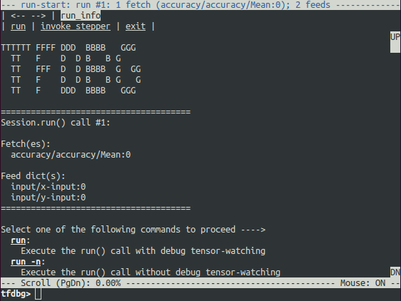 - -This is what we refer to as the *run-start CLI*. It lists the feeds and fetches -to the current `Session.run` call, before executing anything. - -If the screen size is too small to display the content of the message in its -entirety, you can resize it. - -Use the **PageUp** / **PageDown** / **Home** / **End** keys to navigate the -screen output. On most keyboards lacking those keys **Fn + Up** / -**Fn + Down** / **Fn + Right** / **Fn + Left** will work. - -Enter the `run` command (or just `r`) at the command prompt: - -``` -tfdbg> run -``` - -The `run` command causes tfdbg to execute until the end of the next -`Session.run()` call, which calculates the model's accuracy using a test data -set. tfdbg augments the runtime Graph to dump all intermediate tensors. -After the run ends, tfdbg displays all the dumped tensors values in the -*run-end CLI*. For example: - -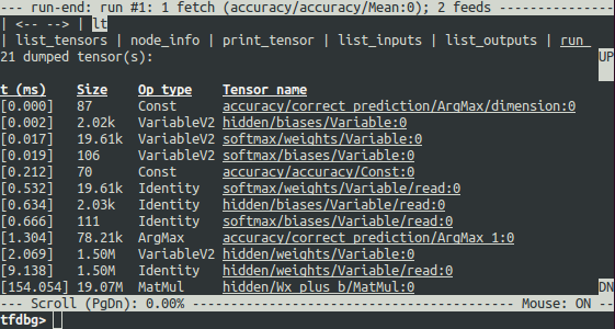 - -This list of tensors can also be obtained by running the command `lt` after you -executed `run`. - -### tfdbg CLI Frequently-Used Commands - -Try the following commands at the `tfdbg>` prompt (referencing the code at -`tensorflow/python/debug/examples/debug_mnist.py`): - -| Command | Syntax or Option | Explanation | Example | -|:-------------------|:---------------- |:------------ |:------------------------- | -| **`lt`** | | **List dumped tensors.** | `lt` | -| | `-n <name_pattern>` | List dumped tensors with names matching given regular-expression pattern. | `lt -n Softmax.*` | -| | `-t <op_pattern>` | List dumped tensors with op types matching given regular-expression pattern. | `lt -t MatMul` | -| | `-f <filter_name>` | List only the tensors that pass a registered tensor filter. | `lt -f has_inf_or_nan` | -| | `-f <filter_name> -fenn <regex>` | List only the tensors that pass a registered tensor filter, excluding nodes with names matching the regular expression. | `lt -f has_inf_or_nan` `-fenn .*Sqrt.*` | -| | `-s <sort_key>` | Sort the output by given `sort_key`, whose possible values are `timestamp` (default), `dump_size`, `op_type` and `tensor_name`. | `lt -s dump_size` | -| | `-r` | Sort in reverse order. | `lt -r -s dump_size` | -| **`pt`** | | **Print value of a dumped tensor.** | | -| | `pt <tensor>` | Print tensor value. | `pt hidden/Relu:0` | -| | `pt <tensor>[slicing]` | Print a subarray of tensor, using [numpy](http://www.numpy.org/)-style array slicing. | `pt hidden/Relu:0[0:50,:]` | -| | `-a` | Print the entirety of a large tensor, without using ellipses. (May take a long time for large tensors.) | `pt -a hidden/Relu:0[0:50,:]` | -| | `-r <range>` | Highlight elements falling into specified numerical range. Multiple ranges can be used in conjunction. | `pt hidden/Relu:0 -a -r [[-inf,-1],[1,inf]]` | -| | `-n <number>` | Print dump corresponding to specified 0-based dump number. Required for tensors with multiple dumps. | `pt -n 0 hidden/Relu:0` | -| | `-s` | Include a summary of the numeric values of the tensor (applicable only to non-empty tensors with Boolean and numeric types such as `int*` and `float*`.) | `pt -s hidden/Relu:0[0:50,:]` | -| | `-w` | Write the value of the tensor (possibly sliced) to a Numpy file using [`numpy.save()`](https://docs.scipy.org/doc/numpy-1.13.0/reference/generated/numpy.save.html) | `pt -s hidden/Relu:0 -w /tmp/relu.npy` | -| **`@[coordinates]`** | | Navigate to specified element in `pt` output. | `@[10,0]` or `@10,0` | -| **`/regex`** | | [less](https://linux.die.net/man/1/less)-style search for given regular expression. | `/inf` | -| **`/`** | | Scroll to the next line with matches to the searched regex (if any). | `/` | -| **`pf`** | | **Print a value in the feed_dict to `Session.run`.** | | -| | `pf <feed_tensor_name>` | Print the value of the feed. Also note that the `pf` command has the `-a`, `-r` and `-s` flags (not listed below), which have the same syntax and semantics as the identically-named flags of `pt`. | `pf input_xs:0` | -| **eval** | | **Evaluate arbitrary Python and numpy expression.** | | -| | `eval <expression>` | Evaluate a Python / numpy expression, with numpy available as `np` and debug tensor names enclosed in backticks. | ``eval "np.matmul((`output/Identity:0` / `Softmax:0`).T, `Softmax:0`)"`` | -| | `-a` | Print a large-sized evaluation result in its entirety, i.e., without using ellipses. | ``eval -a 'np.sum(`Softmax:0`, axis=1)'`` | -| | `-w` | Write the result of the evaluation to a Numpy file using [`numpy.save()`](https://docs.scipy.org/doc/numpy-1.13.0/reference/generated/numpy.save.html) | ``eval -a 'np.sum(`Softmax:0`, axis=1)' -w /tmp/softmax_sum.npy`` | -| **`ni`** | | **Display node information.** | | -| | `-a` | Include node attributes in the output. | `ni -a hidden/Relu` | -| | `-d` | List the debug dumps available from the node. | `ni -d hidden/Relu` | -| | `-t` | Display the Python stack trace of the node's creation. | `ni -t hidden/Relu` | -| **`li`** | | **List inputs to node** | | -| | `-r` | List the inputs to node, recursively (the input tree.) | `li -r hidden/Relu:0` | -| | `-d <max_depth>` | Limit recursion depth under the `-r` mode. | `li -r -d 3 hidden/Relu:0` | -| | `-c` | Include control inputs. | `li -c -r hidden/Relu:0` | -| | `-t` | Show op types of input nodes. | `li -t -r hidden/Relu:0` | -| **`lo`** | | **List output recipients of node** | | -| | `-r` | List the output recipients of node, recursively (the output tree.) | `lo -r hidden/Relu:0` | -| | `-d <max_depth>` | Limit recursion depth under the `-r` mode. | `lo -r -d 3 hidden/Relu:0` | -| | `-c` | Include recipients via control edges. | `lo -c -r hidden/Relu:0` | -| | `-t` | Show op types of recipient nodes. | `lo -t -r hidden/Relu:0` | -| **`ls`** | | **List Python source files involved in node creation.** | | -| | `-p <path_pattern>` | Limit output to source files matching given regular-expression path pattern. | `ls -p .*debug_mnist.*` | -| | `-n` | Limit output to node names matching given regular-expression pattern. | `ls -n Softmax.*` | -| **`ps`** | | **Print Python source file.** | | -| | `ps <file_path>` | Print given Python source file source.py, with the lines annotated with the nodes created at each of them (if any). | `ps /path/to/source.py` | -| | `-t` | Perform annotation with respect to Tensors, instead of the default, nodes. | `ps -t /path/to/source.py` | -| | `-b <line_number>` | Annotate source.py beginning at given line. | `ps -b 30 /path/to/source.py` | -| | `-m <max_elements>` | Limit the number of elements in the annotation for each line. | `ps -m 100 /path/to/source.py` | -| **`run`** | | **Proceed to the next Session.run()** | `run` | -| | `-n` | Execute through the next `Session.run` without debugging, and drop to CLI right before the run after that. | `run -n` | -| | `-t <T>` | Execute `Session.run` `T - 1` times without debugging, followed by a run with debugging. Then drop to CLI right after the debugged run. | `run -t 10` | -| | `-f <filter_name>` | Continue executing `Session.run` until any intermediate tensor triggers the specified Tensor filter (causes the filter to return `True`). | `run -f has_inf_or_nan` | -| | `-f <filter_name> -fenn <regex>` | Continue executing `Session.run` until any intermediate tensor whose node names doesn't match the regular expression triggers the specified Tensor filter (causes the filter to return `True`). | `run -f has_inf_or_nan -fenn .*Sqrt.*` | -| | `--node_name_filter <pattern>` | Execute the next `Session.run`, watching only nodes with names matching the given regular-expression pattern. | `run --node_name_filter Softmax.*` | -| | `--op_type_filter <pattern>` | Execute the next `Session.run`, watching only nodes with op types matching the given regular-expression pattern. | `run --op_type_filter Variable.*` | -| | `--tensor_dtype_filter <pattern>` | Execute the next `Session.run`, dumping only Tensors with data types (`dtype`s) matching the given regular-expression pattern. | `run --tensor_dtype_filter int.*` | -| | `-p` | Execute the next `Session.run` call in profiling mode. | `run -p` | -| **`ri`** | | **Display information about the run the current run, including fetches and feeds.** | `ri` | -| **`config`** | | **Set or show persistent TFDBG UI configuration.** | | -| | `set` | Set the value of a config item: {`graph_recursion_depth`, `mouse_mode`}. | `config set graph_recursion_depth 3` | -| | `show` | Show current persistent UI configuration. | `config show` | -| **`version`** | | **Print the version of TensorFlow and its key dependencies.** | `version` | -| **`help`** | | **Print general help information** | `help` | -| | `help <command>` | Print help for given command. | `help lt` | - -Note that each time you enter a command, a new screen output -will appear. This is somewhat analogous to web pages in a browser. You can -navigate between these screens by clicking the `<--` and -`-->` text arrows near the top-left corner of the CLI. - -### Other Features of the tfdbg CLI - -In addition to the commands listed above, the tfdbg CLI provides the following -additional features: - -* To navigate through previous tfdbg commands, type in a few characters - followed by the Up or Down arrow keys. tfdbg will show you the history of - commands that started with those characters. -* To navigate through the history of screen outputs, do either of the - following: - * Use the `prev` and `next` commands. - * Click underlined `<--` and `-->` links near the top left corner of the - screen. -* Tab completion of commands and some command arguments. -* To redirect the screen output to a file instead of the screen, end the - command with bash-style redirection. For example, the following command - redirects the output of the pt command to the `/tmp/xent_value_slices.txt` - file: - - ```none - tfdbg> pt cross_entropy/Log:0[:, 0:10] > /tmp/xent_value_slices.txt - ``` - -### Finding `nan`s and `inf`s - -In this first `Session.run()` call, there happen to be no problematic numerical -values. You can move on to the next run by using the command `run` or its -shorthand `r`. - -> TIP: If you enter `run` or `r` repeatedly, you will be able to move through -> the `Session.run()` calls in a sequential manner. -> -> You can also use the `-t` flag to move ahead a number of `Session.run()` calls -> at a time, for example: -> -> ``` -> tfdbg> run -t 10 -> ``` - -Instead of entering `run` repeatedly and manually searching for `nan`s and -`inf`s in the run-end UI after every `Session.run()` call (for example, by using -the `pt` command shown in the table above) , you can use the following -command to let the debugger repeatedly execute `Session.run()` calls without -stopping at the run-start or run-end prompt, until the first `nan` or `inf` -value shows up in the graph. This is analogous to *conditional breakpoints* in -some procedural-language debuggers: - -```none -tfdbg> run -f has_inf_or_nan -``` - -> NOTE: The preceding command works properly because a tensor filter called -> `has_inf_or_nan` has been registered for you when the wrapped session is -> created. This filter detects `nan`s and `inf`s (as explained previously). -> If you have registered any other filters, you can -> use "run -f" to have tfdbg run until any tensor triggers that filter (cause -> the filter to return True). -> -> ``` python -> def my_filter_callable(datum, tensor): -> # A filter that detects zero-valued scalars. -> return len(tensor.shape) == 0 and tensor == 0.0 -> -> sess.add_tensor_filter('my_filter', my_filter_callable) -> ``` -> -> Then at the tfdbg run-start prompt run until your filter is triggered: -> -> ``` -> tfdbg> run -f my_filter -> ``` - -See [this API document](https://www.tensorflow.org/api_docs/python/tfdbg/DebugDumpDir#find) -for more information on the expected signature and return value of the predicate -`Callable` used with `add_tensor_filter()`. - -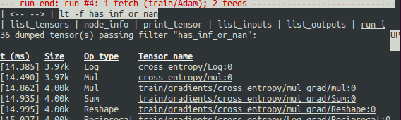 - -As the screen display indicates on the first line, the `has_inf_or_nan` filter is first triggered -during the fourth `Session.run()` call: an -[Adam optimizer](https://www.tensorflow.org/api_docs/python/tf/train/AdamOptimizer) -forward-backward training pass on the graph. In this run, 36 (out of the total -95) intermediate tensors contain `nan` or `inf` values. These tensors are listed -in chronological order, with their timestamps displayed on the left. At the top -of the list, you can see the first tensor in which the bad numerical values -first surfaced: `cross_entropy/Log:0`. - -To view the value of the tensor, click the underlined tensor name -`cross_entropy/Log:0` or enter the equivalent command: - -```none -tfdbg> pt cross_entropy/Log:0 -``` - -Scroll down a little and you will notice some scattered `inf` values. If the -instances of `inf` and `nan` are difficult to spot by eye, you can use the -following command to perform a regex search and highlight the output: - -```none -tfdbg> /inf -``` - -Or, alternatively: - -```none -tfdbg> /(inf|nan) -``` - -You can also use the `-s` or `--numeric_summary` command to get a quick summary -of the types of numeric values in the tensor: - -``` none -tfdbg> pt -s cross_entropy/Log:0 -``` - -From the summary, you can see that several of the 1000 elements of the -`cross_entropy/Log:0` tensor are `-inf`s (negative infinities). - -Why did these infinities appear? To further debug, display more information -about the node `cross_entropy/Log` by clicking the underlined `node_info` menu -item on the top or entering the equivalent node_info (`ni`) command: - -```none -tfdbg> ni cross_entropy/Log -``` - - - -You can see that this node has the op type `Log` -and that its input is the node `Softmax`. Run the following command to -take a closer look at the input tensor: - -```none -tfdbg> pt Softmax:0 -``` - -Examine the values in the input tensor, searching for zeros: - -```none -tfdbg> /0\.000 -``` - -Indeed, there are zeros. Now it is clear that the origin of the bad numerical -values is the node `cross_entropy/Log` taking logs of zeros. To find out the -culprit line in the Python source code, use the `-t` flag of the `ni` command -to show the traceback of the node's construction: - -```none -tfdbg> ni -t cross_entropy/Log -``` - -If you click "node_info" at the top of the screen, tfdbg automatically shows the -traceback of the node's construction. - -From the traceback, you can see that the op is constructed at the following -line: -[`debug_mnist.py`](https://www.tensorflow.org/code/tensorflow/python/debug/examples/debug_mnist.py): - -```python -diff = y_ * tf.log(y) -``` - -**tfdbg** has a feature that makes it easy to trace Tensors and ops back to -lines in Python source files. It can annotate lines of a Python file with -the ops or Tensors created by them. To use this feature, -simply click the underlined line numbers in the stack trace output of the -`ni -t <op_name>` commands, or use the `ps` (or `print_source`) command such as: -`ps /path/to/source.py`. For example, the following screenshot shows the output -of a `ps` command. - - - -### Fixing the problem - -To fix the problem, edit `debug_mnist.py`, changing the original line: - -```python -diff = -(y_ * tf.log(y)) -``` - -to the built-in, numerically-stable implementation of softmax cross-entropy: - -```python -diff = tf.losses.softmax_cross_entropy(labels=y_, logits=logits) -``` - -Rerun with the `--debug` flag as follows: - -```none -python -m tensorflow.python.debug.examples.debug_mnist --debug -``` - -At the `tfdbg>` prompt, enter the following command: - -```none -run -f has_inf_or_nan` -``` - -Confirm that no tensors are flagged as containing `nan` or `inf` values, and -accuracy now continues to rise rather than getting stuck. Success! - -## Debugging TensorFlow Estimators - -This section explains how to debug TensorFlow programs that use the `Estimator` -APIs. Part of the convenience provided by these APIs is that -they manage `Session`s internally. This makes the `LocalCLIDebugWrapperSession` -described in the preceding sections inapplicable. Fortunately, you can still -debug them by using special `hook`s provided by `tfdbg`. - -`tfdbg` can debug the -`tf.estimator.Estimator.train`, -`tf.estimator.Estimator.evaluate` and -`tf.estimator.Estimator.predict` -methods of tf-learn `Estimator`s. To debug `Estimator.train()`, -create a `LocalCLIDebugHook` and supply it in the `hooks` argument. For example: - -```python -# First, let your BUILD target depend on "//tensorflow/python/debug:debug_py" -# (You don't need to worry about the BUILD dependency if you are using a pip -# install of open-source TensorFlow.) -from tensorflow.python import debug as tf_debug - -# Create a LocalCLIDebugHook and use it as a monitor when calling fit(). -hooks = [tf_debug.LocalCLIDebugHook()] - -# To debug `train`: -classifier.train(input_fn, - steps=1000, - hooks=hooks) -``` - -Similarly, to debug `Estimator.evaluate()` and `Estimator.predict()`, assign -hooks to the `hooks` parameter, as in the following example: - -```python -# To debug `evaluate`: -accuracy_score = classifier.evaluate(eval_input_fn, - hooks=hooks)["accuracy"] - -# To debug `predict`: -predict_results = classifier.predict(predict_input_fn, hooks=hooks) -``` - -[debug_tflearn_iris.py](https://www.tensorflow.org/code/tensorflow/python/debug/examples/debug_tflearn_iris.py), -contains a full example of how to use the tfdbg with `Estimator`s. -To run this example, do: - -```none -python -m tensorflow.python.debug.examples.debug_tflearn_iris --debug -``` - -The `LocalCLIDebugHook` also allows you to configure a `watch_fn` that can be -used to flexibly specify what `Tensor`s to watch on different `Session.run()` -calls, as a function of the `fetches` and `feed_dict` and other states. See -`tfdbg.DumpingDebugWrapperSession.__init__` -for more details. - -## Debugging Keras Models with TFDBG - -To use TFDBG with -[tf.keras](https://www.tensorflow.org/api_docs/python/tf/keras), -let the Keras backend use a TFDBG-wrapped Session object. For example, to use -the CLI wrapper: - -``` python -import tensorflow as tf -from tensorflow.python import debug as tf_debug - -tf.keras.backend.set_session(tf_debug.LocalCLIDebugWrapperSession(tf.Session())) - -# Define your keras model, called "model". - -# Calls to `fit()`, 'evaluate()` and `predict()` methods will break into the -# TFDBG CLI. -model.fit(...) -model.evaluate(...) -model.predict(...) -``` - -With minor modification, the preceding code example also works for the -[non-TensorFlow version of Keras](https://keras.io/) running against a -TensorFlow backend. You just need to replace `tf.keras.backend` with -`keras.backend`. - -## Debugging tf-slim with TFDBG - -TFDBG supports debugging of training and evaluation with -[tf-slim](https://github.com/tensorflow/tensorflow/tree/master/tensorflow/contrib/slim). -As detailed below, training and evaluation require slightly different debugging -workflows. - -### Debugging training in tf-slim -To debug the training process, provide `LocalCLIDebugWrapperSession` to the -`session_wrapper` argument of `slim.learning.train()`. For example: - -``` python -import tensorflow as tf -from tensorflow.python import debug as tf_debug - -# ... Code that creates the graph and the train_op ... -tf.contrib.slim.learning.train( - train_op, - logdir, - number_of_steps=10, - session_wrapper=tf_debug.LocalCLIDebugWrapperSession) -``` - -### Debugging evaluation in tf-slim -To debug the evaluation process, provide `LocalCLIDebugHook` to the -`hooks` argument of `slim.evaluation.evaluate_once()`. For example: - -``` python -import tensorflow as tf -from tensorflow.python import debug as tf_debug - -# ... Code that creates the graph and the eval and final ops ... -tf.contrib.slim.evaluation.evaluate_once( - '', - checkpoint_path, - logdir, - eval_op=my_eval_op, - final_op=my_value_op, - hooks=[tf_debug.LocalCLIDebugHook()]) -``` - -## Offline Debugging of Remotely-Running Sessions - -Often, your model is running on a remote machine or a process that you don't -have terminal access to. To perform model debugging in such cases, you can use -the `offline_analyzer` binary of `tfdbg` (described below). It operates on -dumped data directories. This can be done to both the lower-level `Session` API -and the higher-level `Estimator` API. - -### Debugging Remote tf.Sessions - -If you interact directly with the `tf.Session` API in `python`, you can -configure the `RunOptions` proto that you call your `Session.run()` method -with, by using the method `tfdbg.watch_graph`. -This will cause the intermediate tensors and runtime graphs to be dumped to a -shared storage location of your choice when the `Session.run()` call occurs -(at the cost of slower performance). For example: - -```python -from tensorflow.python import debug as tf_debug - -# ... Code where your session and graph are set up... - -run_options = tf.RunOptions() -tf_debug.watch_graph( - run_options, - session.graph, - debug_urls=["file:///shared/storage/location/tfdbg_dumps_1"]) -# Be sure to specify different directories for different run() calls. - -session.run(fetches, feed_dict=feeds, options=run_options) -``` - -Later, in an environment that you have terminal access to (for example, a local -computer that can access the shared storage location specified in the code -above), you can load and inspect the data in the dump directory on the shared -storage by using the `offline_analyzer` binary of `tfdbg`. For example: - -```none -python -m tensorflow.python.debug.cli.offline_analyzer \ - --dump_dir=/shared/storage/location/tfdbg_dumps_1 -``` - -The `Session` wrapper `DumpingDebugWrapperSession` offers an easier and more -flexible way to generate file-system dumps that can be analyzed offline. -To use it, simply wrap your session in a `tf_debug.DumpingDebugWrapperSession`. -For example: - -```python -# Let your BUILD target depend on "//tensorflow/python/debug:debug_py -# (You don't need to worry about the BUILD dependency if you are using a pip -# install of open-source TensorFlow.) -from tensorflow.python import debug as tf_debug - -sess = tf_debug.DumpingDebugWrapperSession( - sess, "/shared/storage/location/tfdbg_dumps_1/", watch_fn=my_watch_fn) -``` - -The `watch_fn` argument accepts a `Callable` that allows you to configure what -`tensor`s to watch on different `Session.run()` calls, as a function of the -`fetches` and `feed_dict` to the `run()` call and other states. - -### C++ and other languages - -If your model code is written in C++ or other languages, you can also -modify the `debug_options` field of `RunOptions` to generate debug dumps that -can be inspected offline. See -[the proto definition](https://www.tensorflow.org/code/tensorflow/core/protobuf/debug.proto) -for more details. - -### Debugging Remotely-Running Estimators - -If your remote TensorFlow server runs `Estimator`s, -you can use the non-interactive `DumpingDebugHook`. For example: - -```python -# Let your BUILD target depend on "//tensorflow/python/debug:debug_py -# (You don't need to worry about the BUILD dependency if you are using a pip -# install of open-source TensorFlow.) -from tensorflow.python import debug as tf_debug - -hooks = [tf_debug.DumpingDebugHook("/shared/storage/location/tfdbg_dumps_1")] -``` - -Then this `hook` can be used in the same way as the `LocalCLIDebugHook` examples -described earlier in this document. -As the training, evaluation or prediction happens with `Estimator`, -tfdbg creates directories having the following name pattern: -`/shared/storage/location/tfdbg_dumps_1/run_<epoch_timestamp_microsec>_<uuid>`. -Each directory corresponds to a `Session.run()` call that underlies -the `fit()` or `evaluate()` call. You can load these directories and inspect -them in a command-line interface in an offline manner using the -`offline_analyzer` offered by tfdbg. For example: - -```bash -python -m tensorflow.python.debug.cli.offline_analyzer \ - --dump_dir="/shared/storage/location/tfdbg_dumps_1/run_<epoch_timestamp_microsec>_<uuid>" -``` - -## Frequently Asked Questions - -**Q**: _Do the timestamps on the left side of the `lt` output reflect actual - performance in a non-debugging session?_ - -**A**: No. The debugger inserts additional special-purpose debug nodes to the - graph to record the values of intermediate tensors. These nodes - slow down the graph execution. If you are interested in profiling your - model, check out - - 1. The profiling mode of tfdbg: `tfdbg> run -p`. - 2. [tfprof](https://github.com/tensorflow/tensorflow/tree/master/tensorflow/core/profiler) - and other profiling tools for TensorFlow. - -**Q**: _How do I link tfdbg against my `Session` in Bazel? Why do I see an - error such as "ImportError: cannot import name debug"?_ - -**A**: In your BUILD rule, declare dependencies: - `"//tensorflow:tensorflow_py"` and `"//tensorflow/python/debug:debug_py"`. - The first is the dependency that you include to use TensorFlow even - without debugger support; the second enables the debugger. - Then, In your Python file, add: - -```python -from tensorflow.python import debug as tf_debug - -# Then wrap your TensorFlow Session with the local-CLI wrapper. -sess = tf_debug.LocalCLIDebugWrapperSession(sess) -``` - -**Q**: _Does tfdbg help debug runtime errors such as shape mismatches?_ - -**A**: Yes. tfdbg intercepts errors generated by ops during runtime and presents - the errors with some debug instructions to the user in the CLI. - See examples: - -```none -# Debugging shape mismatch during matrix multiplication. -python -m tensorflow.python.debug.examples.debug_errors \ - --error shape_mismatch --debug - -# Debugging uninitialized variable. -python -m tensorflow.python.debug.examples.debug_errors \ - --error uninitialized_variable --debug -``` - -**Q**: _How can I let my tfdbg-wrapped Sessions or Hooks run the debug mode -only from the main thread?_ - -**A**: -This is a common use case, in which the `Session` object is used from multiple -threads concurrently. Typically, the child threads take care of background tasks -such as running enqueue operations. Often, you want to debug only the main -thread (or less frequently, only one of the child threads). You can use the -`thread_name_filter` keyword argument of `LocalCLIDebugWrapperSession` to -achieve this type of thread-selective debugging. For example, to debug from the -main thread only, construct a wrapped `Session` as follows: - -```python -sess = tf_debug.LocalCLIDebugWrapperSession(sess, thread_name_filter="MainThread$") -``` - -The above example relies on the fact that main threads in Python have the -default name `MainThread`. - -**Q**: _The model I am debugging is very large. The data dumped by tfdbg -fills up the free space of my disk. What can I do?_ - -**A**: -You might encounter this problem in any of the following situations: - -* models with many intermediate tensors -* very large intermediate tensors -* many `tf.while_loop` iterations - -There are three possible workarounds or solutions: - -* The constructors of `LocalCLIDebugWrapperSession` and `LocalCLIDebugHook` - provide a keyword argument, `dump_root`, to specify the path - to which tfdbg dumps the debug data. You can use it to let tfdbg dump the - debug data on a disk with larger free space. For example: - -```python -# For LocalCLIDebugWrapperSession -sess = tf_debug.LocalCLIDebugWrapperSession(dump_root="/with/lots/of/space") - -# For LocalCLIDebugHook -hooks = [tf_debug.LocalCLIDebugHook(dump_root="/with/lots/of/space")] -``` - Make sure that the directory pointed to by dump_root is empty or nonexistent. - `tfdbg` cleans up the dump directories before exiting. - -* Reduce the batch size used during the runs. -* Use the filtering options of tfdbg's `run` command to watch only specific - nodes in the graph. For example: - - ``` - tfdbg> run --node_name_filter .*hidden.* - tfdbg> run --op_type_filter Variable.* - tfdbg> run --tensor_dtype_filter int.* - ``` - - The first command above watches only nodes whose name match the - regular-expression pattern `.*hidden.*`. The second command watches only - operations whose name match the pattern `Variable.*`. The third one watches - only the tensors whose dtype match the pattern `int.*` (e.g., `int32`). - - -**Q**: _Why can't I select text in the tfdbg CLI?_ - -**A**: This is because the tfdbg CLI enables mouse events in the terminal by - default. This [mouse-mask](https://linux.die.net/man/3/mousemask) mode - overrides default terminal interactions, including text selection. You - can re-enable text selection by using the command `mouse off` or - `m off`. - -**Q**: _Why does the tfdbg CLI show no dumped tensors when I debug code like the following?_ - -``` python -a = tf.ones([10], name="a") -b = tf.add(a, a, name="b") -sess = tf.Session() -sess = tf_debug.LocalCLIDebugWrapperSession(sess) -sess.run(b) -``` - -**A**: The reason why you see no data dumped is because every node in the - executed TensorFlow graph is constant-folded by the TensorFlow runtime. - In this example, `a` is a constant tensor; therefore, the fetched - tensor `b` is effectively also a constant tensor. TensorFlow's graph - optimization folds the graph that contains `a` and `b` into a single - node to speed up future runs of the graph, which is why `tfdbg` does - not generate any intermediate tensor dumps. However, if `a` were a - `tf.Variable`, as in the following example: - -``` python -import numpy as np - -a = tf.Variable(np.ones(10), name="a") -b = tf.add(a, a, name="b") -sess = tf.Session() -sess.run(tf.global_variables_initializer()) -sess = tf_debug.LocalCLIDebugWrapperSession(sess) -sess.run(b) -``` - -the constant-folding would not occur and `tfdbg` should show the intermediate -tensor dumps. - - -**Q**: I am debugging a model that generates unwanted infinities or NaNs. But - there are some nodes in my model that are known to generate infinities - or NaNs in their output tensors even under completely normal conditions. - How can I skip those nodes during my `run -f has_inf_or_nan` actions? - -**A**: Use the `--filter_exclude_node_names` (`-fenn` for short) flag. For - example, if you known you have a node with name matching the regular - expression `.*Sqrt.*` that generates infinities or NaNs regardless - of whether the model is behaving correctly, you can exclude the nodes - from the infinity/NaN-finding runs with the command - `run -f has_inf_or_nan -fenn .*Sqrt.*`. - - -**Q**: Is there a GUI for tfdbg? - -**A**: Yes, the **TensorBoard Debugger Plugin** is the GUI of tfdbg. - It offers features such as inspection of the computation graph, - real-time visualization of tensor values, continuation to tensor - and conditional breakpoints, and tying tensors to their - graph-construction source code, all in the browser environment. - To get started, please visit - [its README](https://github.com/tensorflow/tensorboard/blob/master/tensorboard/plugins/debugger/README.md). diff --git a/tensorflow/docs_src/guide/eager.md b/tensorflow/docs_src/guide/eager.md deleted file mode 100644 index 3b5797a638..0000000000 --- a/tensorflow/docs_src/guide/eager.md +++ /dev/null @@ -1,854 +0,0 @@ -# Eager Execution - -TensorFlow's eager execution is an imperative programming environment that -evaluates operations immediately, without building graphs: operations return -concrete values instead of constructing a computational graph to run later. This -makes it easy to get started with TensorFlow and debug models, and it -reduces boilerplate as well. To follow along with this guide, run the code -samples below in an interactive `python` interpreter. - -Eager execution is a flexible machine learning platform for research and -experimentation, providing: - -* *An intuitive interface*—Structure your code naturally and use Python data - structures. Quickly iterate on small models and small data. -* *Easier debugging*—Call ops directly to inspect running models and test - changes. Use standard Python debugging tools for immediate error reporting. -* *Natural control flow*—Use Python control flow instead of graph control - flow, simplifying the specification of dynamic models. - -Eager execution supports most TensorFlow operations and GPU acceleration. For a -collection of examples running in eager execution, see: -[tensorflow/contrib/eager/python/examples](https://github.com/tensorflow/tensorflow/tree/master/tensorflow/contrib/eager/python/examples). - -Note: Some models may experience increased overhead with eager execution -enabled. Performance improvements are ongoing, but please -[file a bug](https://github.com/tensorflow/tensorflow/issues) if you find a -problem and share your benchmarks. - -## Setup and basic usage - -Upgrade to the latest version of TensorFlow: - -``` -$ pip install --upgrade tensorflow -``` - -To start eager execution, add `tf.enable_eager_execution()` to the beginning of -the program or console session. Do not add this operation to other modules that -the program calls. - -```py -from __future__ import absolute_import, division, print_function - -import tensorflow as tf - -tf.enable_eager_execution() -``` - -Now you can run TensorFlow operations and the results will return immediately: - -```py -tf.executing_eagerly() # => True - -x = [[2.]] -m = tf.matmul(x, x) -print("hello, {}".format(m)) # => "hello, [[4.]]" -``` - -Enabling eager execution changes how TensorFlow operations behave—now they -immediately evaluate and return their values to Python. `tf.Tensor` objects -reference concrete values instead of symbolic handles to nodes in a computational -graph. Since there isn't a computational graph to build and run later in a -session, it's easy to inspect results using `print()` or a debugger. Evaluating, -printing, and checking tensor values does not break the flow for computing -gradients. - -Eager execution works nicely with [NumPy](http://www.numpy.org/). NumPy -operations accept `tf.Tensor` arguments. TensorFlow -[math operations](https://www.tensorflow.org/api_guides/python/math_ops) convert -Python objects and NumPy arrays to `tf.Tensor` objects. The -`tf.Tensor.numpy` method returns the object's value as a NumPy `ndarray`. - -```py -a = tf.constant([[1, 2], - [3, 4]]) -print(a) -# => tf.Tensor([[1 2] -# [3 4]], shape=(2, 2), dtype=int32) - -# Broadcasting support -b = tf.add(a, 1) -print(b) -# => tf.Tensor([[2 3] -# [4 5]], shape=(2, 2), dtype=int32) - -# Operator overloading is supported -print(a * b) -# => tf.Tensor([[ 2 6] -# [12 20]], shape=(2, 2), dtype=int32) - -# Use NumPy values -import numpy as np - -c = np.multiply(a, b) -print(c) -# => [[ 2 6] -# [12 20]] - -# Obtain numpy value from a tensor: -print(a.numpy()) -# => [[1 2] -# [3 4]] -``` - -The `tf.contrib.eager` module contains symbols available to both eager and graph execution -environments and is useful for writing code to [work with graphs](#work_with_graphs): - -```py -tfe = tf.contrib.eager -``` - -## Dynamic control flow - -A major benefit of eager execution is that all the functionality of the host -language is available while your model is executing. So, for example, -it is easy to write [fizzbuzz](https://en.wikipedia.org/wiki/Fizz_buzz): - -```py -def fizzbuzz(max_num): - counter = tf.constant(0) - max_num = tf.convert_to_tensor(max_num) - for num in range(max_num.numpy()): - num = tf.constant(num) - if int(num % 3) == 0 and int(num % 5) == 0: - print('FizzBuzz') - elif int(num % 3) == 0: - print('Fizz') - elif int(num % 5) == 0: - print('Buzz') - else: - print(num) - counter += 1 - return counter -``` - -This has conditionals that depend on tensor values and it prints these values -at runtime. - -## Build a model - -Many machine learning models are represented by composing layers. When -using TensorFlow with eager execution you can either write your own layers or -use a layer provided in the `tf.keras.layers` package. - -While you can use any Python object to represent a layer, -TensorFlow has `tf.keras.layers.Layer` as a convenient base class. Inherit from -it to implement your own layer: - -```py -class MySimpleLayer(tf.keras.layers.Layer): - def __init__(self, output_units): - super(MySimpleLayer, self).__init__() - self.output_units = output_units - - def build(self, input_shape): - # The build method gets called the first time your layer is used. - # Creating variables on build() allows you to make their shape depend - # on the input shape and hence removes the need for the user to specify - # full shapes. It is possible to create variables during __init__() if - # you already know their full shapes. - self.kernel = self.add_variable( - "kernel", [input_shape[-1], self.output_units]) - - def call(self, input): - # Override call() instead of __call__ so we can perform some bookkeeping. - return tf.matmul(input, self.kernel) -``` - -Use `tf.keras.layers.Dense` layer instead of `MySimpleLayer` above as it has -a superset of its functionality (it can also add a bias). - -When composing layers into models you can use `tf.keras.Sequential` to represent -models which are a linear stack of layers. It is easy to use for basic models: - -```py -model = tf.keras.Sequential([ - tf.keras.layers.Dense(10, input_shape=(784,)), # must declare input shape - tf.keras.layers.Dense(10) -]) -``` - -Alternatively, organize models in classes by inheriting from `tf.keras.Model`. -This is a container for layers that is a layer itself, allowing `tf.keras.Model` -objects to contain other `tf.keras.Model` objects. - -```py -class MNISTModel(tf.keras.Model): - def __init__(self): - super(MNISTModel, self).__init__() - self.dense1 = tf.keras.layers.Dense(units=10) - self.dense2 = tf.keras.layers.Dense(units=10) - - def call(self, input): - """Run the model.""" - result = self.dense1(input) - result = self.dense2(result) - result = self.dense2(result) # reuse variables from dense2 layer - return result - -model = MNISTModel() -``` - -It's not required to set an input shape for the `tf.keras.Model` class since -the parameters are set the first time input is passed to the layer. - -`tf.keras.layers` classes create and contain their own model variables that -are tied to the lifetime of their layer objects. To share layer variables, share -their objects. - - -## Eager training - -### Computing gradients - -[Automatic differentiation](https://en.wikipedia.org/wiki/Automatic_differentiation) -is useful for implementing machine learning algorithms such as -[backpropagation](https://en.wikipedia.org/wiki/Backpropagation) for training -neural networks. During eager execution, use `tf.GradientTape` to trace -operations for computing gradients later. - -`tf.GradientTape` is an opt-in feature to provide maximal performance when -not tracing. Since different operations can occur during each call, all -forward-pass operations get recorded to a "tape". To compute the gradient, play -the tape backwards and then discard. A particular `tf.GradientTape` can only -compute one gradient; subsequent calls throw a runtime error. - -```py -w = tf.Variable([[1.0]]) -with tf.GradientTape() as tape: - loss = w * w - -grad = tape.gradient(loss, w) -print(grad) # => tf.Tensor([[ 2.]], shape=(1, 1), dtype=float32) -``` - -Here's an example of `tf.GradientTape` that records forward-pass operations -to train a simple model: - -```py -# A toy dataset of points around 3 * x + 2 -NUM_EXAMPLES = 1000 -training_inputs = tf.random_normal([NUM_EXAMPLES]) -noise = tf.random_normal([NUM_EXAMPLES]) -training_outputs = training_inputs * 3 + 2 + noise - -def prediction(input, weight, bias): - return input * weight + bias - -# A loss function using mean-squared error -def loss(weights, biases): - error = prediction(training_inputs, weights, biases) - training_outputs - return tf.reduce_mean(tf.square(error)) - -# Return the derivative of loss with respect to weight and bias -def grad(weights, biases): - with tf.GradientTape() as tape: - loss_value = loss(weights, biases) - return tape.gradient(loss_value, [weights, biases]) - -train_steps = 200 -learning_rate = 0.01 -# Start with arbitrary values for W and B on the same batch of data -W = tf.Variable(5.) -B = tf.Variable(10.) - -print("Initial loss: {:.3f}".format(loss(W, B))) - -for i in range(train_steps): - dW, dB = grad(W, B) - W.assign_sub(dW * learning_rate) - B.assign_sub(dB * learning_rate) - if i % 20 == 0: - print("Loss at step {:03d}: {:.3f}".format(i, loss(W, B))) - -print("Final loss: {:.3f}".format(loss(W, B))) -print("W = {}, B = {}".format(W.numpy(), B.numpy())) -``` - -Output (exact numbers may vary): - -``` -Initial loss: 71.204 -Loss at step 000: 68.333 -Loss at step 020: 30.222 -Loss at step 040: 13.691 -Loss at step 060: 6.508 -Loss at step 080: 3.382 -Loss at step 100: 2.018 -Loss at step 120: 1.422 -Loss at step 140: 1.161 -Loss at step 160: 1.046 -Loss at step 180: 0.996 -Final loss: 0.974 -W = 3.01582956314, B = 2.1191945076 -``` - -Replay the `tf.GradientTape` to compute the gradients and apply them in a -training loop. This is demonstrated in an excerpt from the -[mnist_eager.py](https://github.com/tensorflow/models/blob/master/official/mnist/mnist_eager.py) -example: - -```py -dataset = tf.data.Dataset.from_tensor_slices((data.train.images, - data.train.labels)) -... -for (batch, (images, labels)) in enumerate(dataset): - ... - with tf.GradientTape() as tape: - logits = model(images, training=True) - loss_value = loss(logits, labels) - ... - grads = tape.gradient(loss_value, model.variables) - optimizer.apply_gradients(zip(grads, model.variables), - global_step=tf.train.get_or_create_global_step()) -``` - - -The following example creates a multi-layer model that classifies the standard -MNIST handwritten digits. It demonstrates the optimizer and layer APIs to build -trainable graphs in an eager execution environment. - -### Train a model - -Even without training, call the model and inspect the output in eager execution: - -```py -# Create a tensor representing a blank image -batch = tf.zeros([1, 1, 784]) -print(batch.shape) # => (1, 1, 784) - -result = model(batch) -# => tf.Tensor([[[ 0. 0., ..., 0.]]], shape=(1, 1, 10), dtype=float32) -``` - -This example uses the -[dataset.py module](https://github.com/tensorflow/models/blob/master/official/mnist/dataset.py) -from the -[TensorFlow MNIST example](https://github.com/tensorflow/models/tree/master/official/mnist); -download this file to your local directory. Run the following to download the -MNIST data files to your working directory and prepare a `tf.data.Dataset` -for training: - -```py -import dataset # download dataset.py file -dataset_train = dataset.train('./datasets').shuffle(60000).repeat(4).batch(32) -``` - -To train a model, define a loss function to optimize and then calculate -gradients. Use an optimizer to update the variables: - -```py -def loss(model, x, y): - prediction = model(x) - return tf.losses.sparse_softmax_cross_entropy(labels=y, logits=prediction) - -def grad(model, inputs, targets): - with tf.GradientTape() as tape: - loss_value = loss(model, inputs, targets) - return tape.gradient(loss_value, model.variables) - -optimizer = tf.train.GradientDescentOptimizer(learning_rate=0.001) - -x, y = iter(dataset_train).next() -print("Initial loss: {:.3f}".format(loss(model, x, y))) - -# Training loop -for (i, (x, y)) in enumerate(dataset_train): - # Calculate derivatives of the input function with respect to its parameters. - grads = grad(model, x, y) - # Apply the gradient to the model - optimizer.apply_gradients(zip(grads, model.variables), - global_step=tf.train.get_or_create_global_step()) - if i % 200 == 0: - print("Loss at step {:04d}: {:.3f}".format(i, loss(model, x, y))) - -print("Final loss: {:.3f}".format(loss(model, x, y))) -``` - -Output (exact numbers may vary): - -``` -Initial loss: 2.674 -Loss at step 0000: 2.593 -Loss at step 0200: 2.143 -Loss at step 0400: 2.009 -Loss at step 0600: 2.103 -Loss at step 0800: 1.621 -Loss at step 1000: 1.695 -... -Loss at step 6600: 0.602 -Loss at step 6800: 0.557 -Loss at step 7000: 0.499 -Loss at step 7200: 0.744 -Loss at step 7400: 0.681 -Final loss: 0.670 -``` - -And for faster training, move the computation to a GPU: - -```py -with tf.device("/gpu:0"): - for (i, (x, y)) in enumerate(dataset_train): - # minimize() is equivalent to the grad() and apply_gradients() calls. - optimizer.minimize(lambda: loss(model, x, y), - global_step=tf.train.get_or_create_global_step()) -``` - -### Variables and optimizers - -`tf.Variable` objects store mutable `tf.Tensor` values accessed during -training to make automatic differentiation easier. The parameters of a model can -be encapsulated in classes as variables. - -Better encapsulate model parameters by using `tf.Variable` with -`tf.GradientTape`. For example, the automatic differentiation example above -can be rewritten: - -```py -class Model(tf.keras.Model): - def __init__(self): - super(Model, self).__init__() - self.W = tf.Variable(5., name='weight') - self.B = tf.Variable(10., name='bias') - def call(self, inputs): - return inputs * self.W + self.B - -# A toy dataset of points around 3 * x + 2 -NUM_EXAMPLES = 2000 -training_inputs = tf.random_normal([NUM_EXAMPLES]) -noise = tf.random_normal([NUM_EXAMPLES]) -training_outputs = training_inputs * 3 + 2 + noise - -# The loss function to be optimized -def loss(model, inputs, targets): - error = model(inputs) - targets - return tf.reduce_mean(tf.square(error)) - -def grad(model, inputs, targets): - with tf.GradientTape() as tape: - loss_value = loss(model, inputs, targets) - return tape.gradient(loss_value, [model.W, model.B]) - -# Define: -# 1. A model. -# 2. Derivatives of a loss function with respect to model parameters. -# 3. A strategy for updating the variables based on the derivatives. -model = Model() -optimizer = tf.train.GradientDescentOptimizer(learning_rate=0.01) - -print("Initial loss: {:.3f}".format(loss(model, training_inputs, training_outputs))) - -# Training loop -for i in range(300): - grads = grad(model, training_inputs, training_outputs) - optimizer.apply_gradients(zip(grads, [model.W, model.B]), - global_step=tf.train.get_or_create_global_step()) - if i % 20 == 0: - print("Loss at step {:03d}: {:.3f}".format(i, loss(model, training_inputs, training_outputs))) - -print("Final loss: {:.3f}".format(loss(model, training_inputs, training_outputs))) -print("W = {}, B = {}".format(model.W.numpy(), model.B.numpy())) -``` - -Output (exact numbers may vary): - -``` -Initial loss: 69.066 -Loss at step 000: 66.368 -Loss at step 020: 30.107 -Loss at step 040: 13.959 -Loss at step 060: 6.769 -Loss at step 080: 3.567 -Loss at step 100: 2.141 -Loss at step 120: 1.506 -Loss at step 140: 1.223 -Loss at step 160: 1.097 -Loss at step 180: 1.041 -Loss at step 200: 1.016 -Loss at step 220: 1.005 -Loss at step 240: 1.000 -Loss at step 260: 0.998 -Loss at step 280: 0.997 -Final loss: 0.996 -W = 2.99431324005, B = 2.02129220963 -``` - -## Use objects for state during eager execution - -With graph execution, program state (such as the variables) is stored in global -collections and their lifetime is managed by the `tf.Session` object. In -contrast, during eager execution the lifetime of state objects is determined by -the lifetime of their corresponding Python object. - -### Variables are objects - -During eager execution, variables persist until the last reference to the object -is removed, and is then deleted. - -```py -with tf.device("gpu:0"): - v = tf.Variable(tf.random_normal([1000, 1000])) - v = None # v no longer takes up GPU memory -``` - -### Object-based saving - -`tf.train.Checkpoint` can save and restore `tf.Variable`s to and from -checkpoints: - -```py -x = tf.Variable(10.) - -checkpoint = tf.train.Checkpoint(x=x) # save as "x" - -x.assign(2.) # Assign a new value to the variables and save. -save_path = checkpoint.save('./ckpt/') - -x.assign(11.) # Change the variable after saving. - -# Restore values from the checkpoint -checkpoint.restore(save_path) - -print(x) # => 2.0 -``` - -To save and load models, `tf.train.Checkpoint` stores the internal state of objects, -without requiring hidden variables. To record the state of a `model`, -an `optimizer`, and a global step, pass them to a `tf.train.Checkpoint`: - -```py -model = MyModel() -optimizer = tf.train.AdamOptimizer(learning_rate=0.001) -checkpoint_dir = ‘/path/to/model_dir’ -checkpoint_prefix = os.path.join(checkpoint_dir, "ckpt") -root = tf.train.Checkpoint(optimizer=optimizer, - model=model, - optimizer_step=tf.train.get_or_create_global_step()) - -root.save(file_prefix=checkpoint_prefix) -# or -root.restore(tf.train.latest_checkpoint(checkpoint_dir)) -``` - -### Object-oriented metrics - -`tfe.metrics` are stored as objects. Update a metric by passing the new data to -the callable, and retrieve the result using the `tfe.metrics.result` method, -for example: - -```py -m = tfe.metrics.Mean("loss") -m(0) -m(5) -m.result() # => 2.5 -m([8, 9]) -m.result() # => 5.5 -``` - -#### Summaries and TensorBoard - -[TensorBoard](../guide/summaries_and_tensorboard.md) is a visualization tool for -understanding, debugging and optimizing the model training process. It uses -summary events that are written while executing the program. - -`tf.contrib.summary` is compatible with both eager and graph execution -environments. Summary operations, such as `tf.contrib.summary.scalar`, are -inserted during model construction. For example, to record summaries once every -100 global steps: - -```py -global_step = tf.train.get_or_create_global_step() -writer = tf.contrib.summary.create_file_writer(logdir) -writer.set_as_default() - -for _ in range(iterations): - global_step.assign_add(1) - # Must include a record_summaries method - with tf.contrib.summary.record_summaries_every_n_global_steps(100): - # your model code goes here - tf.contrib.summary.scalar('loss', loss) - ... -``` - -## Advanced automatic differentiation topics - -### Dynamic models - -`tf.GradientTape` can also be used in dynamic models. This example for a -[backtracking line search](https://wikipedia.org/wiki/Backtracking_line_search) -algorithm looks like normal NumPy code, except there are gradients and is -differentiable, despite the complex control flow: - -```py -def line_search_step(fn, init_x, rate=1.0): - with tf.GradientTape() as tape: - # Variables are automatically recorded, but manually watch a tensor - tape.watch(init_x) - value = fn(init_x) - grad = tape.gradient(value, init_x) - grad_norm = tf.reduce_sum(grad * grad) - init_value = value - while value > init_value - rate * grad_norm: - x = init_x - rate * grad - value = fn(x) - rate /= 2.0 - return x, value -``` - -### Additional functions to compute gradients - -`tf.GradientTape` is a powerful interface for computing gradients, but there -is another [Autograd](https://github.com/HIPS/autograd)-style API available for -automatic differentiation. These functions are useful if writing math code with -only tensors and gradient functions, and without `tf.Variables`: - -* `tfe.gradients_function` —Returns a function that computes the derivatives - of its input function parameter with respect to its arguments. The input - function parameter must return a scalar value. When the returned function is - invoked, it returns a list of `tf.Tensor` objects: one element for each - argument of the input function. Since anything of interest must be passed as a - function parameter, this becomes unwieldy if there's a dependency on many - trainable parameters. -* `tfe.value_and_gradients_function` —Similar to - `tfe.gradients_function`, but when the returned function is invoked, it - returns the value from the input function in addition to the list of - derivatives of the input function with respect to its arguments. - -In the following example, `tfe.gradients_function` takes the `square` -function as an argument and returns a function that computes the partial -derivatives of `square` with respect to its inputs. To calculate the derivative -of `square` at `3`, `grad(3.0)` returns `6`. - -```py -def square(x): - return tf.multiply(x, x) - -grad = tfe.gradients_function(square) - -square(3.) # => 9.0 -grad(3.) # => [6.0] - -# The second-order derivative of square: -gradgrad = tfe.gradients_function(lambda x: grad(x)[0]) -gradgrad(3.) # => [2.0] - -# The third-order derivative is None: -gradgradgrad = tfe.gradients_function(lambda x: gradgrad(x)[0]) -gradgradgrad(3.) # => [None] - - -# With flow control: -def abs(x): - return x if x > 0. else -x - -grad = tfe.gradients_function(abs) - -grad(3.) # => [1.0] -grad(-3.) # => [-1.0] -``` - -### Custom gradients - -Custom gradients are an easy way to override gradients in eager and graph -execution. Within the forward function, define the gradient with respect to the -inputs, outputs, or intermediate results. For example, here's an easy way to clip -the norm of the gradients in the backward pass: - -```py -@tf.custom_gradient -def clip_gradient_by_norm(x, norm): - y = tf.identity(x) - def grad_fn(dresult): - return [tf.clip_by_norm(dresult, norm), None] - return y, grad_fn -``` - -Custom gradients are commonly used to provide a numerically stable gradient for a -sequence of operations: - -```py -def log1pexp(x): - return tf.log(1 + tf.exp(x)) -grad_log1pexp = tfe.gradients_function(log1pexp) - -# The gradient computation works fine at x = 0. -grad_log1pexp(0.) # => [0.5] - -# However, x = 100 fails because of numerical instability. -grad_log1pexp(100.) # => [nan] -``` - -Here, the `log1pexp` function can be analytically simplified with a custom -gradient. The implementation below reuses the value for `tf.exp(x)` that is -computed during the forward pass—making it more efficient by eliminating -redundant calculations: - -```py -@tf.custom_gradient -def log1pexp(x): - e = tf.exp(x) - def grad(dy): - return dy * (1 - 1 / (1 + e)) - return tf.log(1 + e), grad - -grad_log1pexp = tfe.gradients_function(log1pexp) - -# As before, the gradient computation works fine at x = 0. -grad_log1pexp(0.) # => [0.5] - -# And the gradient computation also works at x = 100. -grad_log1pexp(100.) # => [1.0] -``` - -## Performance - -Computation is automatically offloaded to GPUs during eager execution. If you -want control over where a computation runs you can enclose it in a -`tf.device('/gpu:0')` block (or the CPU equivalent): - -```py -import time - -def measure(x, steps): - # TensorFlow initializes a GPU the first time it's used, exclude from timing. - tf.matmul(x, x) - start = time.time() - for i in range(steps): - x = tf.matmul(x, x) - # tf.matmul can return before completing the matrix multiplication - # (e.g., can return after enqueing the operation on a CUDA stream). - # The x.numpy() call below will ensure that all enqueued operations - # have completed (and will also copy the result to host memory, - # so we're including a little more than just the matmul operation - # time). - _ = x.numpy() - end = time.time() - return end - start - -shape = (1000, 1000) -steps = 200 -print("Time to multiply a {} matrix by itself {} times:".format(shape, steps)) - -# Run on CPU: -with tf.device("/cpu:0"): - print("CPU: {} secs".format(measure(tf.random_normal(shape), steps))) - -# Run on GPU, if available: -if tfe.num_gpus() > 0: - with tf.device("/gpu:0"): - print("GPU: {} secs".format(measure(tf.random_normal(shape), steps))) -else: - print("GPU: not found") -``` - -Output (exact numbers depend on hardware): - -``` -Time to multiply a (1000, 1000) matrix by itself 200 times: -CPU: 1.46628093719 secs -GPU: 0.0593810081482 secs -``` - -A `tf.Tensor` object can be copied to a different device to execute its -operations: - -```py -x = tf.random_normal([10, 10]) - -x_gpu0 = x.gpu() -x_cpu = x.cpu() - -_ = tf.matmul(x_cpu, x_cpu) # Runs on CPU -_ = tf.matmul(x_gpu0, x_gpu0) # Runs on GPU:0 - -if tfe.num_gpus() > 1: - x_gpu1 = x.gpu(1) - _ = tf.matmul(x_gpu1, x_gpu1) # Runs on GPU:1 -``` - -### Benchmarks - -For compute-heavy models, such as -[ResNet50](https://github.com/tensorflow/tensorflow/tree/master/tensorflow/contrib/eager/python/examples/resnet50) -training on a GPU, eager execution performance is comparable to graph execution. -But this gap grows larger for models with less computation and there is work to -be done for optimizing hot code paths for models with lots of small operations. - - -## Work with graphs - -While eager execution makes development and debugging more interactive, -TensorFlow graph execution has advantages for distributed training, performance -optimizations, and production deployment. However, writing graph code can feel -different than writing regular Python code and more difficult to debug. - -For building and training graph-constructed models, the Python program first -builds a graph representing the computation, then invokes `Session.run` to send -the graph for execution on the C++-based runtime. This provides: - -* Automatic differentiation using static autodiff. -* Simple deployment to a platform independent server. -* Graph-based optimizations (common subexpression elimination, constant-folding, etc.). -* Compilation and kernel fusion. -* Automatic distribution and replication (placing nodes on the distributed system). - -Deploying code written for eager execution is more difficult: either generate a -graph from the model, or run the Python runtime and code directly on the server. - -### Write compatible code - -The same code written for eager execution will also build a graph during graph -execution. Do this by simply running the same code in a new Python session where -eager execution is not enabled. - -Most TensorFlow operations work during eager execution, but there are some things -to keep in mind: - -* Use `tf.data` for input processing instead of queues. It's faster and easier. -* Use object-oriented layer APIs—like `tf.keras.layers` and - `tf.keras.Model`—since they have explicit storage for variables. -* Most model code works the same during eager and graph execution, but there are - exceptions. (For example, dynamic models using Python control flow to change the - computation based on inputs.) -* Once eager execution is enabled with `tf.enable_eager_execution`, it - cannot be turned off. Start a new Python session to return to graph execution. - -It's best to write code for both eager execution *and* graph execution. This -gives you eager's interactive experimentation and debuggability with the -distributed performance benefits of graph execution. - -Write, debug, and iterate in eager execution, then import the model graph for -production deployment. Use `tf.train.Checkpoint` to save and restore model -variables, this allows movement between eager and graph execution environments. -See the examples in: -[tensorflow/contrib/eager/python/examples](https://github.com/tensorflow/tensorflow/tree/master/tensorflow/contrib/eager/python/examples). - -### Use eager execution in a graph environment - -Selectively enable eager execution in a TensorFlow graph environment using -`tfe.py_func`. This is used when `tf.enable_eager_execution()` has *not* -been called. - -```py -def my_py_func(x): - x = tf.matmul(x, x) # You can use tf ops - print(x) # but it's eager! - return x - -with tf.Session() as sess: - x = tf.placeholder(dtype=tf.float32) - # Call eager function in graph! - pf = tfe.py_func(my_py_func, [x], tf.float32) - sess.run(pf, feed_dict={x: [[2.0]]}) # [[4.0]] -``` diff --git a/tensorflow/docs_src/guide/embedding.md b/tensorflow/docs_src/guide/embedding.md deleted file mode 100644 index 6007e6847b..0000000000 --- a/tensorflow/docs_src/guide/embedding.md +++ /dev/null @@ -1,262 +0,0 @@ -# Embeddings - -This document introduces the concept of embeddings, gives a simple example of -how to train an embedding in TensorFlow, and explains how to view embeddings -with the TensorBoard Embedding Projector -([live example](http://projector.tensorflow.org)). The first two parts target -newcomers to machine learning or TensorFlow, and the Embedding Projector how-to -is for users at all levels. - -An alternative tutorial on these concepts is available in the -[Embeddings section of Machine Learning Crash Course](https://developers.google.com/machine-learning/crash-course/embeddings/video-lecture). - -[TOC] - -An **embedding** is a mapping from discrete objects, such as words, to vectors -of real numbers. For example, a 300-dimensional embedding for English words -could include: - -``` -blue: (0.01359, 0.00075997, 0.24608, ..., -0.2524, 1.0048, 0.06259) -blues: (0.01396, 0.11887, -0.48963, ..., 0.033483, -0.10007, 0.1158) -orange: (-0.24776, -0.12359, 0.20986, ..., 0.079717, 0.23865, -0.014213) -oranges: (-0.35609, 0.21854, 0.080944, ..., -0.35413, 0.38511, -0.070976) -``` - -The individual dimensions in these vectors typically have no inherent meaning. -Instead, it's the overall patterns of location and distance between vectors -that machine learning takes advantage of. - -Embeddings are important for input to machine learning. Classifiers, and neural -networks more generally, work on vectors of real numbers. They train best on -dense vectors, where all values contribute to define an object. However, many -important inputs to machine learning, such as words of text, do not have a -natural vector representation. Embedding functions are the standard and -effective way to transform such discrete input objects into useful -continuous vectors. - -Embeddings are also valuable as outputs of machine learning. Because embeddings -map objects to vectors, applications can use similarity in vector space (for -instance, Euclidean distance or the angle between vectors) as a robust and -flexible measure of object similarity. One common use is to find nearest -neighbors. Using the same word embeddings as above, for instance, here are the -three nearest neighbors for each word and the corresponding angles: - -``` -blue: (red, 47.6°), (yellow, 51.9°), (purple, 52.4°) -blues: (jazz, 53.3°), (folk, 59.1°), (bluegrass, 60.6°) -orange: (yellow, 53.5°), (colored, 58.0°), (bright, 59.9°) -oranges: (apples, 45.3°), (lemons, 48.3°), (mangoes, 50.4°) -``` - -This would tell an application that apples and oranges are in some way more -similar (45.3° apart) than lemons and oranges (48.3° apart). - -## Embeddings in TensorFlow - -To create word embeddings in TensorFlow, we first split the text into words -and then assign an integer to every word in the vocabulary. Let us assume that -this has already been done, and that `word_ids` is a vector of these integers. -For example, the sentence “I have a cat.” could be split into -`[“I”, “have”, “a”, “cat”, “.”]` and then the corresponding `word_ids` tensor -would have shape `[5]` and consist of 5 integers. To map these word ids -to vectors, we need to create the embedding variable and use the -`tf.nn.embedding_lookup` function as follows: - -``` -word_embeddings = tf.get_variable(“word_embeddings”, - [vocabulary_size, embedding_size]) -embedded_word_ids = tf.nn.embedding_lookup(word_embeddings, word_ids) -``` - -After this, the tensor `embedded_word_ids` will have shape `[5, embedding_size]` -in our example and contain the embeddings (dense vectors) for each of the 5 -words. At the end of training, `word_embeddings` will contain the embeddings -for all words in the vocabulary. - -Embeddings can be trained in many network types, and with various loss -functions and data sets. For example, one could use a recurrent neural network -to predict the next word from the previous one given a large corpus of -sentences, or one could train two networks to do multi-lingual translation. -These methods are described in the [Vector Representations of Words](../tutorials/representation/word2vec.md) -tutorial. - -## Visualizing Embeddings - -TensorBoard includes the **Embedding Projector**, a tool that lets you -interactively visualize embeddings. This tool can read embeddings from your -model and render them in two or three dimensions. - -The Embedding Projector has three panels: - -- *Data panel* on the top left, where you can choose the run, the embedding - variable and data columns to color and label points by. -- *Projections panel* on the bottom left, where you can choose the type of - projection. -- *Inspector panel* on the right side, where you can search for particular - points and see a list of nearest neighbors. - -### Projections -The Embedding Projector provides three ways to reduce the dimensionality of a -data set. - -- *[t-SNE](https://en.wikipedia.org/wiki/T-distributed_stochastic_neighbor_embedding)*: - a nonlinear nondeterministic algorithm (T-distributed stochastic neighbor - embedding) that tries to preserve local neighborhoods in the data, often at - the expense of distorting global structure. You can choose whether to compute - two- or three-dimensional projections. - -- *[PCA](https://en.wikipedia.org/wiki/Principal_component_analysis)*: - a linear deterministic algorithm (principal component analysis) that tries to - capture as much of the data variability in as few dimensions as possible. PCA - tends to highlight large-scale structure in the data, but can distort local - neighborhoods. The Embedding Projector computes the top 10 principal - components, from which you can choose two or three to view. - -- *Custom*: a linear projection onto horizontal and vertical axes that you - specify using labels in the data. You define the horizontal axis, for - instance, by giving text patterns for "Left" and "Right". The Embedding - Projector finds all points whose label matches the "Left" pattern and - computes the centroid of that set; similarly for "Right". The line passing - through these two centroids defines the horizontal axis. The vertical axis is - likewise computed from the centroids for points matching the "Up" and "Down" - text patterns. - -Further useful articles are -[How to Use t-SNE Effectively](https://distill.pub/2016/misread-tsne/) and -[Principal Component Analysis Explained Visually](http://setosa.io/ev/principal-component-analysis/). - -### Exploration - -You can explore visually by zooming, rotating, and panning using natural -click-and-drag gestures. Hovering your mouse over a point will show any -[metadata](#metadata) for that point. You can also inspect nearest-neighbor -subsets. Clicking on a point causes the right pane to list the nearest -neighbors, along with distances to the current point. The nearest-neighbor -points are also highlighted in the projection. - -It is sometimes useful to restrict the view to a subset of points and perform -projections only on those points. To do so, you can select points in multiple -ways: - -- After clicking on a point, its nearest neighbors are also selected. -- After a search, the points matching the query are selected. -- Enabling selection, clicking on a point and dragging defines a selection - sphere. - -Then click the "Isolate *nnn* points" button at the top of the Inspector pane -on the right hand side. The following image shows 101 points selected and ready -for the user to click "Isolate 101 points": - - - -*Selection of the nearest neighbors of “important” in a word embedding dataset.* - -Advanced tip: filtering with custom projection can be powerful. Below, we -filtered the 100 nearest neighbors of “politics” and projected them onto the -“worst” - “best” vector as an x axis. The y axis is random. As a result, one -finds on the right side “ideas”, “science”, “perspective”, “journalism” but on -the left “crisis”, “violence” and “conflict”. - -<table width="100%;"> - <tr> - <td style="width: 30%;"> - <img src="https://www.tensorflow.org/images/embedding-custom-controls.png" alt="Custom controls panel" title="Custom controls panel" /> - </td> - <td style="width: 70%;"> - <img src="https://www.tensorflow.org/images/embedding-custom-projection.png" alt="Custom projection" title="Custom projection" /> - </td> - </tr> - <tr> - <td style="width: 30%;"> - Custom projection controls. - </td> - <td style="width: 70%;"> - Custom projection of neighbors of "politics" onto "best" - "worst" vector. - </td> - </tr> -</table> - -To share your findings, you can use the bookmark panel in the bottom right -corner and save the current state (including computed coordinates of any -projection) as a small file. The Projector can then be pointed to a set of one -or more of these files, producing the panel below. Other users can then walk -through a sequence of bookmarks. - -<img src="https://www.tensorflow.org/images/embedding-bookmark.png" alt="Bookmark panel" style="width:300px;"> - -### Metadata - -If you are working with an embedding, you'll probably want to attach -labels/images to the data points. You can do this by generating a metadata file -containing the labels for each point and clicking "Load data" in the data panel -of the Embedding Projector. - -The metadata can be either labels or images, which are -stored in a separate file. For labels, the format should -be a [TSV file](https://en.wikipedia.org/wiki/Tab-separated_values) -(tab characters shown in red) whose first line contains column headers -(shown in bold) and subsequent lines contain the metadata values. For example: - -<code> -<b>Word<span style="color:#800;">\t</span>Frequency</b><br/> - Airplane<span style="color:#800;">\t</span>345<br/> - Car<span style="color:#800;">\t</span>241<br/> - ... -</code> - -The order of lines in the metadata file is assumed to match the order of -vectors in the embedding variable, except for the header. Consequently, the -(i+1)-th line in the metadata file corresponds to the i-th row of the embedding -variable. If the TSV metadata file has only a single column, then we don’t -expect a header row, and assume each row is the label of the embedding. We -include this exception because it matches the commonly-used "vocab file" -format. - -To use images as metadata, you must produce a single -[sprite image](https://www.google.com/webhp#q=what+is+a+sprite+image), -consisting of small thumbnails, one for each vector in the embedding. The -sprite should store thumbnails in row-first order: the first data point placed -in the top left and the last data point in the bottom right, though the last -row doesn't have to be filled, as shown below. - -<table style="border: none;"> -<tr style="background-color: transparent;"> - <td style="border: 1px solid black">0</td> - <td style="border: 1px solid black">1</td> - <td style="border: 1px solid black">2</td> -</tr> -<tr style="background-color: transparent;"> - <td style="border: 1px solid black">3</td> - <td style="border: 1px solid black">4</td> - <td style="border: 1px solid black">5</td> -</tr> -<tr style="background-color: transparent;"> - <td style="border: 1px solid black">6</td> - <td style="border: 1px solid black">7</td> - <td style="border: 1px solid black"></td> -</tr> -</table> - -Follow [this link](https://www.tensorflow.org/images/embedding-mnist.mp4) -to see a fun example of thumbnail images in the Embedding Projector. - - -## Mini-FAQ - -**Is "embedding" an action or a thing?** -Both. People talk about embedding words in a vector space (action) and about -producing word embeddings (things). Common to both is the notion of embedding -as a mapping from discrete objects to vectors. Creating or applying that -mapping is an action, but the mapping itself is a thing. - -**Are embeddings high-dimensional or low-dimensional?** -It depends. A 300-dimensional vector space of words and phrases, for instance, -is often called low-dimensional (and dense) when compared to the millions of -words and phrases it can contain. But mathematically it is high-dimensional, -displaying many properties that are dramatically different from what our human -intuition has learned about 2- and 3-dimensional spaces. - -**Is an embedding the same as an embedding layer?** -No. An *embedding layer* is a part of neural network, but an *embedding* is a more -general concept. diff --git a/tensorflow/docs_src/guide/estimators.md b/tensorflow/docs_src/guide/estimators.md deleted file mode 100644 index 3903bfd126..0000000000 --- a/tensorflow/docs_src/guide/estimators.md +++ /dev/null @@ -1,196 +0,0 @@ -# Estimators - -This document introduces `tf.estimator`--a high-level TensorFlow -API that greatly simplifies machine learning programming. Estimators encapsulate -the following actions: - -* training -* evaluation -* prediction -* export for serving - -You may either use the pre-made Estimators we provide or write your -own custom Estimators. All Estimators--whether pre-made or custom--are -classes based on the `tf.estimator.Estimator` class. - -For a quick example try [Estimator tutorials]](../tutorials/estimators/linear). -To see each sub-topic in depth, see the [Estimator guides](premade_estimators). - -Note: TensorFlow also includes a deprecated `Estimator` class at -`tf.contrib.learn.Estimator`, which you should not use. - - -## Advantages of Estimators - -Estimators provide the following benefits: - -* You can run Estimator-based models on a local host or on a - distributed multi-server environment without changing your model. - Furthermore, you can run Estimator-based models on CPUs, GPUs, - or TPUs without recoding your model. -* Estimators simplify sharing implementations between model developers. -* You can develop a state of the art model with high-level intuitive code. - In short, it is generally much easier to create models with Estimators - than with the low-level TensorFlow APIs. -* Estimators are themselves built on `tf.keras.layers`, which - simplifies customization. -* Estimators build the graph for you. -* Estimators provide a safe distributed training loop that controls how and - when to: - * build the graph - * initialize variables - * load data - * handle exceptions - * create checkpoint files and recover from failures - * save summaries for TensorBoard - -When writing an application with Estimators, you must separate the data input -pipeline from the model. This separation simplifies experiments with -different data sets. - - -## Pre-made Estimators - -Pre-made Estimators enable you to work at a much higher conceptual level -than the base TensorFlow APIs. You no longer have to worry about creating -the computational graph or sessions since Estimators handle all -the "plumbing" for you. That is, pre-made Estimators create and manage -`tf.Graph` and `tf.Session` objects for you. Furthermore, -pre-made Estimators let you experiment with different model architectures by -making only minimal code changes. `tf.estimator.DNNClassifier`, -for example, is a pre-made Estimator class that trains classification models -based on dense, feed-forward neural networks. - - -### Structure of a pre-made Estimators program - -A TensorFlow program relying on a pre-made Estimator typically consists -of the following four steps: - -1. **Write one or more dataset importing functions.** For example, you might - create one function to import the training set and another function to - import the test set. Each dataset importing function must return two - objects: - - * a dictionary in which the keys are feature names and the - values are Tensors (or SparseTensors) containing the corresponding - feature data - * a Tensor containing one or more labels - - For example, the following code illustrates the basic skeleton for - an input function: - - def input_fn(dataset): - ... # manipulate dataset, extracting the feature dict and the label - return feature_dict, label - - (See [Importing Data](../guide/datasets.md) for full details.) - -2. **Define the feature columns.** Each `tf.feature_column` - identifies a feature name, its type, and any input pre-processing. - For example, the following snippet creates three feature - columns that hold integer or floating-point data. The first two - feature columns simply identify the feature's name and type. The - third feature column also specifies a lambda the program will invoke - to scale the raw data: - - # Define three numeric feature columns. - population = tf.feature_column.numeric_column('population') - crime_rate = tf.feature_column.numeric_column('crime_rate') - median_education = tf.feature_column.numeric_column('median_education', - normalizer_fn=lambda x: x - global_education_mean) - -3. **Instantiate the relevant pre-made Estimator.** For example, here's - a sample instantiation of a pre-made Estimator named `LinearClassifier`: - - # Instantiate an estimator, passing the feature columns. - estimator = tf.estimator.LinearClassifier( - feature_columns=[population, crime_rate, median_education], - ) - -4. **Call a training, evaluation, or inference method.** - For example, all Estimators provide a `train` method, which trains a model. - - # my_training_set is the function created in Step 1 - estimator.train(input_fn=my_training_set, steps=2000) - - -### Benefits of pre-made Estimators - -Pre-made Estimators encode best practices, providing the following benefits: - -* Best practices for determining where different parts of the computational - graph should run, implementing strategies on a single machine or on a - cluster. -* Best practices for event (summary) writing and universally useful - summaries. - -If you don't use pre-made Estimators, you must implement the preceding -features yourself. - - -## Custom Estimators - -The heart of every Estimator--whether pre-made or custom--is its -**model function**, which is a method that builds graphs for training, -evaluation, and prediction. When you are using a pre-made Estimator, -someone else has already implemented the model function. When relying -on a custom Estimator, you must write the model function yourself. A -[companion document](../guide/custom_estimators.md) -explains how to write the model function. - - -## Recommended workflow - -We recommend the following workflow: - -1. Assuming a suitable pre-made Estimator exists, use it to build your - first model and use its results to establish a baseline. -2. Build and test your overall pipeline, including the integrity and - reliability of your data with this pre-made Estimator. -3. If suitable alternative pre-made Estimators are available, run - experiments to determine which pre-made Estimator produces the - best results. -4. Possibly, further improve your model by building your own custom Estimator. - - -## Creating Estimators from Keras models - -You can convert existing Keras models to Estimators. Doing so enables your Keras -model to access Estimator's strengths, such as distributed training. Call -`tf.keras.estimator.model_to_estimator` as in the -following sample: - -```python -# Instantiate a Keras inception v3 model. -keras_inception_v3 = tf.keras.applications.inception_v3.InceptionV3(weights=None) -# Compile model with the optimizer, loss, and metrics you'd like to train with. -keras_inception_v3.compile(optimizer=tf.keras.optimizers.SGD(lr=0.0001, momentum=0.9), - loss='categorical_crossentropy', - metric='accuracy') -# Create an Estimator from the compiled Keras model. Note the initial model -# state of the keras model is preserved in the created Estimator. -est_inception_v3 = tf.keras.estimator.model_to_estimator(keras_model=keras_inception_v3) - -# Treat the derived Estimator as you would with any other Estimator. -# First, recover the input name(s) of Keras model, so we can use them as the -# feature column name(s) of the Estimator input function: -keras_inception_v3.input_names # print out: ['input_1'] -# Once we have the input name(s), we can create the input function, for example, -# for input(s) in the format of numpy ndarray: -train_input_fn = tf.estimator.inputs.numpy_input_fn( - x={"input_1": train_data}, - y=train_labels, - num_epochs=1, - shuffle=False) -# To train, we call Estimator's train function: -est_inception_v3.train(input_fn=train_input_fn, steps=2000) -``` -Note that the names of feature columns and labels of a keras estimator come from -the corresponding compiled keras model. For example, the input key names for -`train_input_fn` above can be obtained from `keras_inception_v3.input_names`, -and similarly, the predicted output names can be obtained from -`keras_inception_v3.output_names`. - -For more details, please refer to the documentation for -`tf.keras.estimator.model_to_estimator`. diff --git a/tensorflow/docs_src/guide/faq.md b/tensorflow/docs_src/guide/faq.md deleted file mode 100644 index a02635ebba..0000000000 --- a/tensorflow/docs_src/guide/faq.md +++ /dev/null @@ -1,296 +0,0 @@ -# Frequently Asked Questions - -This document provides answers to some of the frequently asked questions about -TensorFlow. If you have a question that is not covered here, you might find an -answer on one of the TensorFlow [community resources](../about/index.md). - -[TOC] - -## Features and Compatibility - -#### Can I run distributed training on multiple computers? - -Yes! TensorFlow gained -[support for distributed computation](../deploy/distributed.md) in -version 0.8. TensorFlow now supports multiple devices (CPUs and GPUs) in one or -more computers. - -#### Does TensorFlow work with Python 3? - -As of the 0.6.0 release timeframe (Early December 2015), we do support Python -3.3+. - -## Building a TensorFlow graph - -See also the -[API documentation on building graphs](../api_guides/python/framework.md). - -#### Why does `c = tf.matmul(a, b)` not execute the matrix multiplication immediately? - -In the TensorFlow Python API, `a`, `b`, and `c` are -`tf.Tensor` objects. A `Tensor` object is -a symbolic handle to the result of an operation, but does not actually hold the -values of the operation's output. Instead, TensorFlow encourages users to build -up complicated expressions (such as entire neural networks and its gradients) as -a dataflow graph. You then offload the computation of the entire dataflow graph -(or a subgraph of it) to a TensorFlow -`tf.Session`, which is able to execute the -whole computation much more efficiently than executing the operations -one-by-one. - -#### How are devices named? - -The supported device names are `"/device:CPU:0"` (or `"/cpu:0"`) for the CPU -device, and `"/device:GPU:i"` (or `"/gpu:i"`) for the *i*th GPU device. - -#### How do I place operations on a particular device? - -To place a group of operations on a device, create them within a -`tf.device` context. See -the how-to documentation on -[using GPUs with TensorFlow](../guide/using_gpu.md) for details of how -TensorFlow assigns operations to devices, and the -[CIFAR-10 tutorial](../tutorials/images/deep_cnn.md) for an example model that -uses multiple GPUs. - - -## Running a TensorFlow computation - -See also the -[API documentation on running graphs](../api_guides/python/client.md). - -#### What's the deal with feeding and placeholders? - -Feeding is a mechanism in the TensorFlow Session API that allows you to -substitute different values for one or more tensors at run time. The `feed_dict` -argument to `tf.Session.run` is a -dictionary that maps `tf.Tensor` objects to -numpy arrays (and some other types), which will be used as the values of those -tensors in the execution of a step. - -#### What is the difference between `Session.run()` and `Tensor.eval()`? - -If `t` is a `tf.Tensor` object, -`tf.Tensor.eval` is shorthand for -`tf.Session.run`, where `sess` is the -current `tf.get_default_session`. The -two following snippets of code are equivalent: - -```python -# Using `Session.run()`. -sess = tf.Session() -c = tf.constant(5.0) -print(sess.run(c)) - -# Using `Tensor.eval()`. -c = tf.constant(5.0) -with tf.Session(): - print(c.eval()) -``` - -In the second example, the session acts as a -[context manager](https://docs.python.org/2.7/reference/compound_stmts.html#with), -which has the effect of installing it as the default session for the lifetime of -the `with` block. The context manager approach can lead to more concise code for -simple use cases (like unit tests); if your code deals with multiple graphs and -sessions, it may be more straightforward to make explicit calls to -`Session.run()`. - -#### Do Sessions have a lifetime? What about intermediate tensors? - -Sessions can own resources, such as -`tf.Variable`, -`tf.QueueBase`, and -`tf.ReaderBase`. These resources can sometimes use -a significant amount of memory, and can be released when the session is closed by calling -`tf.Session.close`. - -The intermediate tensors that are created as part of a call to -[`Session.run()`](../api_guides/python/client.md) will be freed at or before the -end of the call. - -#### Does the runtime parallelize parts of graph execution? - -The TensorFlow runtime parallelizes graph execution across many different -dimensions: - -* The individual ops have parallel implementations, using multiple cores in a - CPU, or multiple threads in a GPU. -* Independent nodes in a TensorFlow graph can run in parallel on multiple - devices, which makes it possible to speed up - [CIFAR-10 training using multiple GPUs](../tutorials/images/deep_cnn.md). -* The Session API allows multiple concurrent steps (i.e. calls to - `tf.Session.run` in parallel). This - enables the runtime to get higher throughput, if a single step does not use - all of the resources in your computer. - -#### Which client languages are supported in TensorFlow? - -TensorFlow is designed to support multiple client languages. -Currently, the best-supported client language is [Python](../api_docs/python/index.md). Experimental interfaces for -executing and constructing graphs are also available for -[C++](../api_docs/cc/index.md), [Java](../api_docs/java/reference/org/tensorflow/package-summary.html) and [Go](https://godoc.org/github.com/tensorflow/tensorflow/tensorflow/go). - -TensorFlow also has a -[C-based client API](https://www.tensorflow.org/code/tensorflow/c/c_api.h) -to help build support for more client languages. We invite contributions of new -language bindings. - -Bindings for various other languages (such as [C#](https://github.com/migueldeicaza/TensorFlowSharp), [Julia](https://github.com/malmaud/TensorFlow.jl), [Ruby](https://github.com/somaticio/tensorflow.rb) and [Scala](https://github.com/eaplatanios/tensorflow_scala)) created and supported by the open source community build on top of the C API supported by the TensorFlow maintainers. - -#### Does TensorFlow make use of all the devices (GPUs and CPUs) available on my machine? - -TensorFlow supports multiple GPUs and CPUs. See the how-to documentation on -[using GPUs with TensorFlow](../guide/using_gpu.md) for details of how -TensorFlow assigns operations to devices, and the -[CIFAR-10 tutorial](../tutorials/images/deep_cnn.md) for an example model that -uses multiple GPUs. - -Note that TensorFlow only uses GPU devices with a compute capability greater -than 3.5. - -#### Why does `Session.run()` hang when using a reader or a queue? - -The `tf.ReaderBase` and -`tf.QueueBase` classes provide special operations that -can *block* until input (or free space in a bounded queue) becomes -available. These operations allow you to build sophisticated -[input pipelines](../api_guides/python/reading_data.md), at the cost of making the -TensorFlow computation somewhat more complicated. See the how-to documentation -for -[using `QueueRunner` objects to drive queues and readers](../api_guides/python/reading_data.md#creating_threads_to_prefetch_using_queuerunner_objects) -for more information on how to use them. - -## Variables - -See also the how-to documentation on [variables](../guide/variables.md) and -[the API documentation for variables](../api_guides/python/state_ops.md). - -#### What is the lifetime of a variable? - -A variable is created when you first run the -`tf.Variable.initializer` -operation for that variable in a session. It is destroyed when that -`tf.Session.close`. - -#### How do variables behave when they are concurrently accessed? - -Variables allow concurrent read and write operations. The value read from a -variable may change if it is concurrently updated. By default, concurrent -assignment operations to a variable are allowed to run with no mutual exclusion. -To acquire a lock when assigning to a variable, pass `use_locking=True` to -`tf.Variable.assign`. - -## Tensor shapes - -See also the -`tf.TensorShape`. - -#### How can I determine the shape of a tensor in Python? - -In TensorFlow, a tensor has both a static (inferred) shape and a dynamic (true) -shape. The static shape can be read using the -`tf.Tensor.get_shape` -method: this shape is inferred from the operations that were used to create the -tensor, and may be partially complete (the static-shape may contain `None`). If -the static shape is not fully defined, the dynamic shape of a `tf.Tensor`, `t` -can be determined using `tf.shape(t)`. - -#### What is the difference between `x.set_shape()` and `x = tf.reshape(x)`? - -The `tf.Tensor.set_shape` method updates -the static shape of a `Tensor` object, and it is typically used to provide -additional shape information when this cannot be inferred directly. It does not -change the dynamic shape of the tensor. - -The `tf.reshape` operation creates -a new tensor with a different dynamic shape. - -#### How do I build a graph that works with variable batch sizes? - -It is often useful to build a graph that works with variable batch sizes -so that the same code can be used for (mini-)batch training, and -single-instance inference. The resulting graph can be -`tf.Graph.as_graph_def` -and -`tf.import_graph_def`. - -When building a variable-size graph, the most important thing to remember is not -to encode the batch size as a Python constant, but instead to use a symbolic -`Tensor` to represent it. The following tips may be useful: - -* Use [`batch_size = tf.shape(input)[0]`](../api_docs/python/array_ops.md#shape) - to extract the batch dimension from a `Tensor` called `input`, and store it in - a `Tensor` called `batch_size`. - -* Use `tf.reduce_mean` instead - of `tf.reduce_sum(...) / batch_size`. - - -## TensorBoard - -#### How can I visualize a TensorFlow graph? - -See the [graph visualization tutorial](../guide/graph_viz.md). - -#### What is the simplest way to send data to TensorBoard? - -Add summary ops to your TensorFlow graph, and write -these summaries to a log directory. Then, start TensorBoard using - - python tensorflow/tensorboard/tensorboard.py --logdir=path/to/log-directory - -For more details, see the -[Summaries and TensorBoard tutorial](../guide/summaries_and_tensorboard.md). - -#### Every time I launch TensorBoard, I get a network security popup! - -You can change TensorBoard to serve on localhost rather than '0.0.0.0' by -the flag --host=localhost. This should quiet any security warnings. - -## Extending TensorFlow - -See the how-to documentation for -[adding a new operation to TensorFlow](../extend/adding_an_op.md). - -#### My data is in a custom format. How do I read it using TensorFlow? - -There are three main options for dealing with data in a custom format. - -The easiest option is to write parsing code in Python that transforms the data -into a numpy array. Then, use `tf.data.Dataset.from_tensor_slices` to -create an input pipeline from the in-memory data. - -If your data doesn't fit in memory, try doing the parsing in the Dataset -pipeline. Start with an appropriate file reader, like -`tf.data.TextLineDataset`. Then convert the dataset by mapping -`tf.data.Dataset.map` appropriate operations over it. -Prefer predefined TensorFlow operations such as `tf.decode_raw`, -`tf.decode_csv`, `tf.parse_example`, or `tf.image.decode_png`. - -If your data is not easily parsable with the built-in TensorFlow operations, -consider converting it, offline, to a format that is easily parsable, such -as `tf.python_io.TFRecordWriter` format. - -The most efficient method to customize the parsing behavior is to -[add a new op written in C++](../extend/adding_an_op.md) that parses your -data format. The [guide to handling new data formats](../extend/new_data_formats.md) has -more information about the steps for doing this. - - -## Miscellaneous - -#### What is TensorFlow's coding style convention? - -The TensorFlow Python API adheres to the -[PEP8](https://www.python.org/dev/peps/pep-0008/) conventions.<sup>*</sup> In -particular, we use `CamelCase` names for classes, and `snake_case` names for -functions, methods, and properties. We also adhere to the -[Google Python style guide](https://google.github.io/styleguide/pyguide.html). - -The TensorFlow C++ code base adheres to the -[Google C++ style guide](https://google.github.io/styleguide/cppguide.html). - -(<sup>*</sup> With one exception: we use 2-space indentation instead of 4-space -indentation.) - diff --git a/tensorflow/docs_src/guide/feature_columns.md b/tensorflow/docs_src/guide/feature_columns.md deleted file mode 100644 index 3ad41855e4..0000000000 --- a/tensorflow/docs_src/guide/feature_columns.md +++ /dev/null @@ -1,572 +0,0 @@ -# Feature Columns - -This document details feature columns. Think of **feature columns** as the -intermediaries between raw data and Estimators. Feature columns are very rich, -enabling you to transform a diverse range of raw data into formats that -Estimators can use, allowing easy experimentation. - -In [Premade Estimators](../guide/premade_estimators.md), we used the premade -Estimator, `tf.estimator.DNNClassifier` to train a model to -predict different types of Iris flowers from four input features. That example -created only numerical feature columns (of type -`tf.feature_column.numeric_column`). Although numerical feature columns model -the lengths of petals and sepals effectively, real world data sets contain all -kinds of features, many of which are non-numerical. - -<div style="width:80%; margin:auto; margin-bottom:10px; margin-top:20px;"> -<img style="width:100%" src="../images/feature_columns/feature_cloud.jpg"> -</div> -<div style="text-align: center"> -Some real-world features (such as, longitude) are numerical, but many are not. -</div> - -## Input to a Deep Neural Network - -What kind of data can a deep neural network operate on? The answer -is, of course, numbers (for example, `tf.float32`). After all, every neuron in -a neural network performs multiplication and addition operations on weights and -input data. Real-life input data, however, often contains non-numerical -(categorical) data. For example, consider a `product_class` feature that can -contain the following three non-numerical values: - -* `kitchenware` -* `electronics` -* `sports` - -ML models generally represent categorical values as simple vectors in which a -1 represents the presence of a value and a 0 represents the absence of a value. -For example, when `product_class` is set to `sports`, an ML model would usually -represent `product_class` as `[0, 0, 1]`, meaning: - -* `0`: `kitchenware` is absent -* `0`: `electronics` is absent -* `1`: `sports` is present - -So, although raw data can be numerical or categorical, an ML model represents -all features as numbers. - -## Feature Columns - -As the following figure suggests, you specify the input to a model through the -`feature_columns` argument of an Estimator (`DNNClassifier` for Iris). -Feature Columns bridge input data (as returned by `input_fn`) with your model. - -<div style="width:80%; margin:auto; margin-bottom:10px; margin-top:20px;"> -<img style="width:100%" src="../images/feature_columns/inputs_to_model_bridge.jpg"> -</div> -<div style="text-align: center"> -Feature columns bridge raw data with the data your model needs. -</div> - -To create feature columns, call functions from the -`tf.feature_column` module. This document explains nine of the functions in -that module. As the following figure shows, all nine functions return either a -Categorical-Column or a Dense-Column object, except `bucketized_column`, which -inherits from both classes: - -<div style="width:80%; margin:auto; margin-bottom:10px; margin-top:20px;"> -<img style="width:100%" src="../images/feature_columns/some_constructors.jpg"> -</div> -<div style="text-align: center"> -Feature column methods fall into two main categories and one hybrid category. -</div> - -Let's look at these functions in more detail. - -### Numeric column - -The Iris classifier calls the `tf.feature_column.numeric_column` function for -all input features: - - * `SepalLength` - * `SepalWidth` - * `PetalLength` - * `PetalWidth` - -Although `tf.numeric_column` provides optional arguments, calling -`tf.numeric_column` without any arguments, as follows, is a fine way to specify -a numerical value with the default data type (`tf.float32`) as input to your -model: - -```python -# Defaults to a tf.float32 scalar. -numeric_feature_column = tf.feature_column.numeric_column(key="SepalLength") -``` - -To specify a non-default numerical data type, use the `dtype` argument. For -example: - -``` python -# Represent a tf.float64 scalar. -numeric_feature_column = tf.feature_column.numeric_column(key="SepalLength", - dtype=tf.float64) -``` - -By default, a numeric column creates a single value (scalar). Use the shape -argument to specify another shape. For example: - -<!--TODO(markdaoust) link to full example--> -```python -# Represent a 10-element vector in which each cell contains a tf.float32. -vector_feature_column = tf.feature_column.numeric_column(key="Bowling", - shape=10) - -# Represent a 10x5 matrix in which each cell contains a tf.float32. -matrix_feature_column = tf.feature_column.numeric_column(key="MyMatrix", - shape=[10,5]) -``` -### Bucketized column - -Often, you don't want to feed a number directly into the model, but instead -split its value into different categories based on numerical ranges. To do so, -create a `tf.feature_column.bucketized_column`. For -example, consider raw data that represents the year a house was built. Instead -of representing that year as a scalar numeric column, we could split the year -into the following four buckets: - -<div style="width:80%; margin:auto; margin-bottom:10px; margin-top:20px;"> -<img style="width:100%" src="../images/feature_columns/bucketized_column.jpg"> -</div> -<div style="text-align: center"> -Dividing year data into four buckets. -</div> - -The model will represent the buckets as follows: - -|Date Range |Represented as... | -|:----------|:-----------------| -|< 1960 | [1, 0, 0, 0] | -|>= 1960 but < 1980 | [0, 1, 0, 0] | -|>= 1980 but < 2000 | [0, 0, 1, 0] | -|>= 2000 | [0, 0, 0, 1] | - -Why would you want to split a number—a perfectly valid input to your -model—into a categorical value? Well, notice that the categorization splits a -single input number into a four-element vector. Therefore, the model now can -learn _four individual weights_ rather than just one; four weights creates a -richer model than one weight. More importantly, bucketizing enables the model -to clearly distinguish between different year categories since only one of the -elements is set (1) and the other three elements are cleared (0). For example, -when we just use a single number (a year) as input, a linear model can only -learn a linear relationship. So, bucketing provides the model with additional -flexibility that the model can use to learn. - -The following code demonstrates how to create a bucketized feature: - -<!--TODO(markdaoust) link to full example - housing price grid?--> -```python -# First, convert the raw input to a numeric column. -numeric_feature_column = tf.feature_column.numeric_column("Year") - -# Then, bucketize the numeric column on the years 1960, 1980, and 2000. -bucketized_feature_column = tf.feature_column.bucketized_column( - source_column = numeric_feature_column, - boundaries = [1960, 1980, 2000]) -``` -Note that specifying a _three_-element boundaries vector creates a -_four_-element bucketized vector. - - -### Categorical identity column - -**Categorical identity columns** can be seen as a special case of bucketized -columns. In traditional bucketized columns, each bucket represents a range of -values (for example, from 1960 to 1979). In a categorical identity column, each -bucket represents a single, unique integer. For example, let's say you want to -represent the integer range `[0, 4)`. That is, you want to represent the -integers 0, 1, 2, or 3. In this case, the categorical identity mapping looks -like this: - -<div style="width:80%; margin:auto; margin-bottom:10px; margin-top:20px;"> -<img style="width:100%" src="../images/feature_columns/categorical_column_with_identity.jpg"> -</div> -<div style="text-align: center"> -A categorical identity column mapping. Note that this is a one-hot -encoding, not a binary numerical encoding. -</div> - -As with bucketized columns, a model can learn a separate weight for each class -in a categorical identity column. For example, instead of using a string to -represent the `product_class`, let's represent each class with a unique integer -value. That is: - -* `0="kitchenware"` -* `1="electronics"` -* `2="sport"` - -Call `tf.feature_column.categorical_column_with_identity` to implement a -categorical identity column. For example: - -``` python -# Create categorical output for an integer feature named "my_feature_b", -# The values of my_feature_b must be >= 0 and < num_buckets -identity_feature_column = tf.feature_column.categorical_column_with_identity( - key='my_feature_b', - num_buckets=4) # Values [0, 4) - -# In order for the preceding call to work, the input_fn() must return -# a dictionary containing 'my_feature_b' as a key. Furthermore, the values -# assigned to 'my_feature_b' must belong to the set [0, 4). -def input_fn(): - ... - return ({ 'my_feature_a':[7, 9, 5, 2], 'my_feature_b':[3, 1, 2, 2] }, - [Label_values]) -``` - -### Categorical vocabulary column - -We cannot input strings directly to a model. Instead, we must first map strings -to numeric or categorical values. Categorical vocabulary columns provide a good -way to represent strings as a one-hot vector. For example: - -<div style="width:80%; margin:auto; margin-bottom:10px; margin-top:20px;"> -<img style="width:100%" src="../images/feature_columns/categorical_column_with_vocabulary.jpg"> -</div> -<div style="text-align: center"> -Mapping string values to vocabulary columns. -</div> - -As you can see, categorical vocabulary columns are kind of an enum version of -categorical identity columns. TensorFlow provides two different functions to -create categorical vocabulary columns: - -* `tf.feature_column.categorical_column_with_vocabulary_list` -* `tf.feature_column.categorical_column_with_vocabulary_file` - -`categorical_column_with_vocabulary_list` maps each string to an integer based -on an explicit vocabulary list. For example: - -```python -# Given input "feature_name_from_input_fn" which is a string, -# create a categorical feature by mapping the input to one of -# the elements in the vocabulary list. -vocabulary_feature_column = - tf.feature_column.categorical_column_with_vocabulary_list( - key=feature_name_from_input_fn, - vocabulary_list=["kitchenware", "electronics", "sports"]) -``` - -The preceding function is pretty straightforward, but it has a significant -drawback. Namely, there's way too much typing when the vocabulary list is long. -For these cases, call -`tf.feature_column.categorical_column_with_vocabulary_file` instead, which lets -you place the vocabulary words in a separate file. For example: - -```python - -# Given input "feature_name_from_input_fn" which is a string, -# create a categorical feature to our model by mapping the input to one of -# the elements in the vocabulary file -vocabulary_feature_column = - tf.feature_column.categorical_column_with_vocabulary_file( - key=feature_name_from_input_fn, - vocabulary_file="product_class.txt", - vocabulary_size=3) -``` - -`product_class.txt` should contain one line for each vocabulary element. In our -case: - -```None -kitchenware -electronics -sports -``` - -### Hashed Column - -So far, we've worked with a naively small number of categories. For example, -our product_class example has only 3 categories. Often though, the number of -categories can be so big that it's not possible to have individual categories -for each vocabulary word or integer because that would consume too much memory. -For these cases, we can instead turn the question around and ask, "How many -categories am I willing to have for my input?" In fact, the -`tf.feature_column.categorical_column_with_hash_bucket` function enables you -to specify the number of categories. For this type of feature column the model -calculates a hash value of the input, then puts it into one of -the `hash_bucket_size` categories using the modulo operator, as in the following -pseudocode: - -```python -# pseudocode -feature_id = hash(raw_feature) % hash_bucket_size -``` - -The code to create the `feature_column` might look something like this: - -``` python -hashed_feature_column = - tf.feature_column.categorical_column_with_hash_bucket( - key = "some_feature", - hash_bucket_size = 100) # The number of categories -``` -At this point, you might rightfully think: "This is crazy!" After all, we are -forcing the different input values to a smaller set of categories. This means -that two probably unrelated inputs will be mapped to the same -category, and consequently mean the same thing to the neural network. The -following figure illustrates this dilemma, showing that kitchenware and sports -both get assigned to category (hash bucket) 12: - -<div style="width:80%; margin:auto; margin-bottom:10px; margin-top:20px;"> -<img style="width:100%" src="../images/feature_columns/hashed_column.jpg"> -</div> -<div style="text-align: center"> -Representing data with hash buckets. -</div> - -As with many counterintuitive phenomena in machine learning, it turns out that -hashing often works well in practice. That's because hash categories provide -the model with some separation. The model can use additional features to further -separate kitchenware from sports. - -### Crossed column - -Combining features into a single feature, better known as -[feature crosses](https://developers.google.com/machine-learning/glossary/#feature_cross), -enables the model to learn separate weights for each combination of -features. - -More concretely, suppose we want our model to calculate real estate prices in -Atlanta, GA. Real-estate prices within this city vary greatly depending on -location. Representing latitude and longitude as separate features isn't very -useful in identifying real-estate location dependencies; however, crossing -latitude and longitude into a single feature can pinpoint locations. Suppose we -represent Atlanta as a grid of 100x100 rectangular sections, identifying each -of the 10,000 sections by a feature cross of latitude and longitude. This -feature cross enables the model to train on pricing conditions related to each -individual section, which is a much stronger signal than latitude and longitude -alone. - -The following figure shows our plan, with the latitude & longitude values for -the corners of the city in red text: - -<div style="width:80%; margin:auto; margin-bottom:10px; margin-top:20px;"> -<img style="width:100%" src="../images/feature_columns/Atlanta.jpg"> -</div> -<div style="text-align: center"> -Map of Atlanta. Imagine this map divided into 10,000 sections of -equal size. -</div> - -For the solution, we used a combination of the `bucketized_column` we looked at -earlier, with the `tf.feature_column.crossed_column` function. - -<!--TODO(markdaoust) link to full example--> - -``` python -def make_dataset(latitude, longitude, labels): - assert latitude.shape == longitude.shape == labels.shape - - features = {'latitude': latitude.flatten(), - 'longitude': longitude.flatten()} - labels=labels.flatten() - - return tf.data.Dataset.from_tensor_slices((features, labels)) - - -# Bucketize the latitude and longitude using the `edges` -latitude_bucket_fc = tf.feature_column.bucketized_column( - tf.feature_column.numeric_column('latitude'), - list(atlanta.latitude.edges)) - -longitude_bucket_fc = tf.feature_column.bucketized_column( - tf.feature_column.numeric_column('longitude'), - list(atlanta.longitude.edges)) - -# Cross the bucketized columns, using 5000 hash bins. -crossed_lat_lon_fc = tf.feature_column.crossed_column( - [latitude_bucket_fc, longitude_bucket_fc], 5000) - -fc = [ - latitude_bucket_fc, - longitude_bucket_fc, - crossed_lat_lon_fc] - -# Build and train the Estimator. -est = tf.estimator.LinearRegressor(fc, ...) -``` - -You may create a feature cross from either of the following: - -* Feature names; that is, names from the `dict` returned from `input_fn`. -* Any categorical column, except `categorical_column_with_hash_bucket` - (since `crossed_column` hashes the input). - -When the feature columns `latitude_bucket_fc` and `longitude_bucket_fc` are -crossed, TensorFlow will create `(latitude_fc, longitude_fc)` pairs for each -example. This would produce a full grid of possibilities as follows: - -``` None - (0,0), (0,1)... (0,99) - (1,0), (1,1)... (1,99) - ... ... ... -(99,0), (99,1)...(99, 99) -``` - -Except that a full grid would only be tractable for inputs with limited -vocabularies. Instead of building this, potentially huge, table of inputs, -the `crossed_column` only builds the number requested by the `hash_bucket_size` -argument. The feature column assigns an example to a index by running a hash -function on the tuple of inputs, followed by a modulo operation with -`hash_bucket_size`. - -As discussed earlier, performing the -hash and modulo function limits the number of categories, but can cause category -collisions; that is, multiple (latitude, longitude) feature crosses will end -up in the same hash bucket. In practice though, performing feature crosses -still adds significant value to the learning capability of your models. - -Somewhat counterintuitively, when creating feature crosses, you typically still -should include the original (uncrossed) features in your model (as in the -preceding code snippet). The independent latitude and longitude features help the -model distinguish between examples where a hash collision has occurred in the -crossed feature. - -## Indicator and embedding columns - -Indicator columns and embedding columns never work on features directly, but -instead take categorical columns as input. - -When using an indicator column, we're telling TensorFlow to do exactly what -we've seen in our categorical product_class example. That is, an -**indicator column** treats each category as an element in a one-hot vector, -where the matching category has value 1 and the rest have 0s: - -<div style="width:80%; margin:auto; margin-bottom:10px; margin-top:20px;"> -<img style="width:100%" src="../images/feature_columns/categorical_column_with_identity.jpg"> -</div> -<div style="text-align: center"> -Representing data in indicator columns. -</div> - -Here's how you create an indicator column by calling -`tf.feature_column.indicator_column`: - -``` python -categorical_column = ... # Create any type of categorical column. - -# Represent the categorical column as an indicator column. -indicator_column = tf.feature_column.indicator_column(categorical_column) -``` - -Now, suppose instead of having just three possible classes, we have a million. -Or maybe a billion. For a number of reasons, as the number of categories grow -large, it becomes infeasible to train a neural network using indicator columns. - -We can use an embedding column to overcome this limitation. Instead of -representing the data as a one-hot vector of many dimensions, an -**embedding column** represents that data as a lower-dimensional, ordinary -vector in which each cell can contain any number, not just 0 or 1. By -permitting a richer palette of numbers for every cell, an embedding column -contains far fewer cells than an indicator column. - -Let's look at an example comparing indicator and embedding columns. Suppose our -input examples consist of different words from a limited palette of only 81 -words. Further suppose that the data set provides the following input -words in 4 separate examples: - -* `"dog"` -* `"spoon"` -* `"scissors"` -* `"guitar"` - -In that case, the following figure illustrates the processing path for -embedding columns or indicator columns. - -<div style="width:80%; margin:auto; margin-bottom:10px; margin-top:20px;"> -<img style="width:100%" src="../images/feature_columns/embedding_vs_indicator.jpg"> -</div> -<div style="text-align: center"> -An embedding column stores categorical data in a lower-dimensional -vector than an indicator column. (We just placed random numbers into the -embedding vectors; training determines the actual numbers.) -</div> - -When an example is processed, one of the `categorical_column_with...` functions -maps the example string to a numerical categorical value. For example, a -function maps "spoon" to `[32]`. (The 32 comes from our imagination—the actual -values depend on the mapping function.) You may then represent these numerical -categorical values in either of the following two ways: - -* As an indicator column. A function converts each numeric categorical value - into an 81-element vector (because our palette consists of 81 words), placing - a 1 in the index of the categorical value (0, 32, 79, 80) and a 0 in all the - other positions. - -* As an embedding column. A function uses the numerical categorical values - `(0, 32, 79, 80)` as indices to a lookup table. Each slot in that lookup table - contains a 3-element vector. - -How do the values in the embeddings vectors magically get assigned? Actually, -the assignments happen during training. That is, the model learns the best way -to map your input numeric categorical values to the embeddings vector value in -order to solve your problem. Embedding columns increase your model's -capabilities, since an embeddings vector learns new relationships between -categories from the training data. - -Why is the embedding vector size 3 in our example? Well, the following "formula" -provides a general rule of thumb about the number of embedding dimensions: - -```python -embedding_dimensions = number_of_categories**0.25 -``` - -That is, the embedding vector dimension should be the 4th root of the number of -categories. Since our vocabulary size in this example is 81, the recommended -number of dimensions is 3: - -``` python -3 = 81**0.25 -``` -Note that this is just a general guideline; you can set the number of embedding -dimensions as you please. - -Call `tf.feature_column.embedding_column` to create an `embedding_column` as -suggested by the following snippet: - -``` python -categorical_column = ... # Create any categorical column - -# Represent the categorical column as an embedding column. -# This means creating an embedding vector lookup table with one element for each category. -embedding_column = tf.feature_column.embedding_column( - categorical_column=categorical_column, - dimension=embedding_dimensions) -``` - -[Embeddings](../guide/embedding.md) is a significant topic within machine -learning. This information was just to get you started using them as feature -columns. - -## Passing feature columns to Estimators - -As the following list indicates, not all Estimators permit all types of -`feature_columns` argument(s): - -* `tf.estimator.LinearClassifier` and - `tf.estimator.LinearRegressor`: Accept all types of - feature column. -* `tf.estimator.DNNClassifier` and - `tf.estimator.DNNRegressor`: Only accept dense columns. Other - column types must be wrapped in either an `indicator_column` or - `embedding_column`. -* `tf.estimator.DNNLinearCombinedClassifier` and - `tf.estimator.DNNLinearCombinedRegressor`: - * The `linear_feature_columns` argument accepts any feature column type. - * The `dnn_feature_columns` argument only accepts dense columns. - -## Other Sources - -For more examples on feature columns, view the following: - -* The [Low Level Introduction](../guide/low_level_intro.md#feature_columns) demonstrates how - experiment directly with `feature_columns` using TensorFlow's low level APIs. -* The [Estimator wide and deep learning tutorial](https://github.com/tensorflow/models/tree/master/official/wide_deep) - solves a binary classification problem using `feature_columns` on a variety of - input data types. - -To learn more about embeddings, see the following: - -* [Deep Learning, NLP, and representations](http://colah.github.io/posts/2014-07-NLP-RNNs-Representations/) - (Chris Olah's blog) -* The TensorFlow [Embedding Projector](http://projector.tensorflow.org) diff --git a/tensorflow/docs_src/guide/graph_viz.md b/tensorflow/docs_src/guide/graph_viz.md deleted file mode 100644 index 23f722bbe7..0000000000 --- a/tensorflow/docs_src/guide/graph_viz.md +++ /dev/null @@ -1,317 +0,0 @@ -# TensorBoard: Graph Visualization - -TensorFlow computation graphs are powerful but complicated. The graph visualization can help you understand and debug them. Here's an example of the visualization at work. - - -*Visualization of a TensorFlow graph.* - -To see your own graph, run TensorBoard pointing it to the log directory of the job, click on the graph tab on the top pane and select the appropriate run using the menu at the upper left corner. For in depth information on how to run TensorBoard and make sure you are logging all the necessary information, see [TensorBoard: Visualizing Learning](../guide/summaries_and_tensorboard.md). - -## Name scoping and nodes - -Typical TensorFlow graphs can have many thousands of nodes--far too many to see -easily all at once, or even to lay out using standard graph tools. To simplify, -variable names can be scoped and the visualization uses this information to -define a hierarchy on the nodes in the graph. By default, only the top of this -hierarchy is shown. Here is an example that defines three operations under the -`hidden` name scope using -`tf.name_scope`: - -```python -import tensorflow as tf - -with tf.name_scope('hidden') as scope: - a = tf.constant(5, name='alpha') - W = tf.Variable(tf.random_uniform([1, 2], -1.0, 1.0), name='weights') - b = tf.Variable(tf.zeros([1]), name='biases') -``` - -This results in the following three op names: - -* `hidden/alpha` -* `hidden/weights` -* `hidden/biases` - -By default, the visualization will collapse all three into a node labeled `hidden`. -The extra detail isn't lost. You can double-click, or click -on the orange `+` sign in the top right to expand the node, and then you'll see -three subnodes for `alpha`, `weights` and `biases`. - -Here's a real-life example of a more complicated node in its initial and -expanded states. - -<table width="100%;"> - <tr> - <td style="width: 50%;"> - <img src="https://www.tensorflow.org/images/pool1_collapsed.png" alt="Unexpanded name scope" title="Unexpanded name scope" /> - </td> - <td style="width: 50%;"> - <img src="https://www.tensorflow.org/images/pool1_expanded.png" alt="Expanded name scope" title="Expanded name scope" /> - </td> - </tr> - <tr> - <td style="width: 50%;"> - Initial view of top-level name scope <code>pool_1</code>. Clicking on the orange <code>+</code> button on the top right or double-clicking on the node itself will expand it. - </td> - <td style="width: 50%;"> - Expanded view of <code>pool_1</code> name scope. Clicking on the orange <code>-</code> button on the top right or double-clicking on the node itself will collapse the name scope. - </td> - </tr> -</table> - -Grouping nodes by name scopes is critical to making a legible graph. If you're -building a model, name scopes give you control over the resulting visualization. -**The better your name scopes, the better your visualization.** - -The figure above illustrates a second aspect of the visualization. TensorFlow -graphs have two kinds of connections: data dependencies and control -dependencies. Data dependencies show the flow of tensors between two ops and -are shown as solid arrows, while control dependencies use dotted lines. In the -expanded view (right side of the figure above) all the connections are data -dependencies with the exception of the dotted line connecting `CheckNumerics` -and `control_dependency`. - -There's a second trick to simplifying the layout. Most TensorFlow graphs have a -few nodes with many connections to other nodes. For example, many nodes might -have a control dependency on an initialization step. Drawing all edges between -the `init` node and its dependencies would create a very cluttered view. - -To reduce clutter, the visualization separates out all high-degree nodes to an -*auxiliary* area on the right and doesn't draw lines to represent their edges. -Instead of lines, we draw small *node icons* to indicate the connections. -Separating out the auxiliary nodes typically doesn't remove critical -information since these nodes are usually related to bookkeeping functions. -See [Interaction](#interaction) for how to move nodes between the main graph -and the auxiliary area. - -<table width="100%;"> - <tr> - <td style="width: 50%;"> - <img src="https://www.tensorflow.org/images/conv_1.png" alt="conv_1 is part of the main graph" title="conv_1 is part of the main graph" /> - </td> - <td style="width: 50%;"> - <img src="https://www.tensorflow.org/images/save.png" alt="save is extracted as auxiliary node" title="save is extracted as auxiliary node" /> - </td> - </tr> - <tr> - <td style="width: 50%;"> - Node <code>conv_1</code> is connected to <code>save</code>. Note the little <code>save</code> node icon on its right. - </td> - <td style="width: 50%;"> - <code>save</code> has a high degree, and will appear as an auxiliary node. The connection with <code>conv_1</code> is shown as a node icon on its left. To further reduce clutter, since <code>save</code> has a lot of connections, we show the first 5 and abbreviate the others as <code>... 12 more</code>. - </td> - </tr> -</table> - -One last structural simplification is *series collapsing*. Sequential -motifs--that is, nodes whose names differ by a number at the end and have -isomorphic structures--are collapsed into a single *stack* of nodes, as shown -below. For networks with long sequences, this greatly simplifies the view. As -with hierarchical nodes, double-clicking expands the series. See -[Interaction](#interaction) for how to disable/enable series collapsing for a -specific set of nodes. - -<table width="100%;"> - <tr> - <td style="width: 50%;"> - <img src="https://www.tensorflow.org/images/series.png" alt="Sequence of nodes" title="Sequence of nodes" /> - </td> - <td style="width: 50%;"> - <img src="https://www.tensorflow.org/images/series_expanded.png" alt="Expanded sequence of nodes" title="Expanded sequence of nodes" /> - </td> - </tr> - <tr> - <td style="width: 50%;"> - A collapsed view of a node sequence. - </td> - <td style="width: 50%;"> - A small piece of the expanded view, after double-click. - </td> - </tr> -</table> - -Finally, as one last aid to legibility, the visualization uses special icons -for constants and summary nodes. To summarize, here's a table of node symbols: - -Symbol | Meaning ---- | --- - | *High-level* node representing a name scope. Double-click to expand a high-level node. - | Sequence of numbered nodes that are not connected to each other. - | Sequence of numbered nodes that are connected to each other. - | An individual operation node. - | A constant. - | A summary node. - | Edge showing the data flow between operations. - | Edge showing the control dependency between operations. - | A reference edge showing that the outgoing operation node can mutate the incoming tensor. - -## Interaction {#interaction} - -Navigate the graph by panning and zooming. Click and drag to pan, and use a -scroll gesture to zoom. Double-click on a node, or click on its `+` button, to -expand a name scope that represents a group of operations. To easily keep -track of the current viewpoint when zooming and panning, there is a minimap in -the bottom right corner. - -To close an open node, double-click it again or click its `-` button. You can -also click once to select a node. It will turn a darker color, and details -about it and the nodes it connects to will appear in the info card at upper -right corner of the visualization. - -<table width="100%;"> - <tr> - <td style="width: 50%;"> - <img src="https://www.tensorflow.org/images/infocard.png" alt="Info card of a name scope" title="Info card of a name scope" /> - </td> - <td style="width: 50%;"> - <img src="https://www.tensorflow.org/images/infocard_op.png" alt="Info card of operation node" title="Info card of operation node" /> - </td> - </tr> - <tr> - <td style="width: 50%;"> - Info card showing detailed information for the <code>conv2</code> name scope. The inputs and outputs are combined from the inputs and outputs of the operation nodes inside the name scope. For name scopes no attributes are shown. - </td> - <td style="width: 50%;"> - Info card showing detailed information for the <code>DecodeRaw</code> operation node. In addition to inputs and outputs, the card shows the device and the attributes associated with the current operation. - </td> - </tr> -</table> - -TensorBoard provides several ways to change the visual layout of the graph. This -doesn't change the graph's computational semantics, but it can bring some -clarity to the network's structure. By right clicking on a node or pressing -buttons on the bottom of that node's info card, you can make the following -changes to its layout: - -* Nodes can be moved between the main graph and the auxiliary area. -* A series of nodes can be ungrouped so that the nodes in the series do not -appear grouped together. Ungrouped series can likewise be regrouped. - -Selection can also be helpful in understanding high-degree nodes. Select any -high-degree node, and the corresponding node icons for its other connections -will be selected as well. This makes it easy, for example, to see which nodes -are being saved--and which aren't. - -Clicking on a node name in the info card will select it. If necessary, the -viewpoint will automatically pan so that the node is visible. - -Finally, you can choose two color schemes for your graph, using the color menu -above the legend. The default *Structure View* shows structure: when two -high-level nodes have the same structure, they appear in the same color of the -rainbow. Uniquely structured nodes are gray. There's a second view, which shows -what device the different operations run on. Name scopes are colored -proportionally to the fraction of devices for the operations inside them. - -The images below give an illustration for a piece of a real-life graph. - -<table width="100%;"> - <tr> - <td style="width: 50%;"> - <img src="https://www.tensorflow.org/images/colorby_structure.png" alt="Color by structure" title="Color by structure" /> - </td> - <td style="width: 50%;"> - <img src="https://www.tensorflow.org/images/colorby_device.png" alt="Color by device" title="Color by device" /> - </td> - </tr> - <tr> - <td style="width: 50%;"> - Structure view: The gray nodes have unique structure. The orange <code>conv1</code> and <code>conv2</code> nodes have the same structure, and analogously for nodes with other colors. - </td> - <td style="width: 50%;"> - Device view: Name scopes are colored proportionally to the fraction of devices of the operation nodes inside them. Here, purple means GPU and the green is CPU. - </td> - </tr> -</table> - -## Tensor shape information - -When the serialized `GraphDef` includes tensor shapes, the graph visualizer -labels edges with tensor dimensions, and edge thickness reflects total tensor -size. To include tensor shapes in the `GraphDef` pass the actual graph object -(as in `sess.graph`) to the `FileWriter` when serializing the graph. -The images below show the CIFAR-10 model with tensor shape information: -<table width="100%;"> - <tr> - <td style="width: 100%;"> - <img src="https://www.tensorflow.org/images/tensor_shapes.png" alt="CIFAR-10 model with tensor shape information" title="CIFAR-10 model with tensor shape information" /> - </td> - </tr> - <tr> - <td style="width: 100%;"> - CIFAR-10 model with tensor shape information. - </td> - </tr> -</table> - -## Runtime statistics - -Often it is useful to collect runtime metadata for a run, such as total memory -usage, total compute time, and tensor shapes for nodes. The code example below -is a snippet from the train and test section of a modification of the -[Estimators MNIST tutorial](../tutorials/estimators/cnn.md), in which we have -recorded summaries and -runtime statistics. See the -[Summaries Tutorial](../guide/summaries_and_tensorboard.md#serializing-the-data) -for details on how to record summaries. -Full source is [here](https://www.tensorflow.org/code/tensorflow/examples/tutorials/mnist/mnist_with_summaries.py). - -```python - # Train the model, and also write summaries. - # Every 10th step, measure test-set accuracy, and write test summaries - # All other steps, run train_step on training data, & add training summaries - - def feed_dict(train): - """Make a TensorFlow feed_dict: maps data onto Tensor placeholders.""" - if train or FLAGS.fake_data: - xs, ys = mnist.train.next_batch(100, fake_data=FLAGS.fake_data) - k = FLAGS.dropout - else: - xs, ys = mnist.test.images, mnist.test.labels - k = 1.0 - return {x: xs, y_: ys, keep_prob: k} - - for i in range(FLAGS.max_steps): - if i % 10 == 0: # Record summaries and test-set accuracy - summary, acc = sess.run([merged, accuracy], feed_dict=feed_dict(False)) - test_writer.add_summary(summary, i) - print('Accuracy at step %s: %s' % (i, acc)) - else: # Record train set summaries, and train - if i % 100 == 99: # Record execution stats - run_options = tf.RunOptions(trace_level=tf.RunOptions.FULL_TRACE) - run_metadata = tf.RunMetadata() - summary, _ = sess.run([merged, train_step], - feed_dict=feed_dict(True), - options=run_options, - run_metadata=run_metadata) - train_writer.add_run_metadata(run_metadata, 'step%d' % i) - train_writer.add_summary(summary, i) - print('Adding run metadata for', i) - else: # Record a summary - summary, _ = sess.run([merged, train_step], feed_dict=feed_dict(True)) - train_writer.add_summary(summary, i) -``` - -This code will emit runtime statistics for every 100th step starting at step99. - -When you launch tensorboard and go to the Graph tab, you will now see options -under "Session runs" which correspond to the steps where run metadata was added. -Selecting one of these runs will show you the snapshot of the network at that -step, fading out unused nodes. In the controls on the left hand side, you will -be able to color the nodes by total memory or total compute time. Additionally, -clicking on a node will display the exact total memory, compute time, and -tensor output sizes. - - -<table width="100%;"> - <tr style="height: 380px"> - <td> - <img src="https://www.tensorflow.org/images/colorby_compute_time.png" alt="Color by compute time" title="Color by compute time"/> - </td> - <td> - <img src="https://www.tensorflow.org/images/run_metadata_graph.png" alt="Run metadata graph" title="Run metadata graph" /> - </td> - <td> - <img src="https://www.tensorflow.org/images/run_metadata_infocard.png" alt="Run metadata info card" title="Run metadata info card" /> - </td> - </tr> -</table> diff --git a/tensorflow/docs_src/guide/graphs.md b/tensorflow/docs_src/guide/graphs.md deleted file mode 100644 index c70479dba2..0000000000 --- a/tensorflow/docs_src/guide/graphs.md +++ /dev/null @@ -1,558 +0,0 @@ -# Graphs and Sessions - -TensorFlow uses a **dataflow graph** to represent your computation in terms of -the dependencies between individual operations. This leads to a low-level -programming model in which you first define the dataflow graph, then create a -TensorFlow **session** to run parts of the graph across a set of local and -remote devices. - -This guide will be most useful if you intend to use the low-level programming -model directly. Higher-level APIs such as `tf.estimator.Estimator` and Keras -hide the details of graphs and sessions from the end user, but this guide may -also be useful if you want to understand how these APIs are implemented. - -## Why dataflow graphs? - - - -[Dataflow](https://en.wikipedia.org/wiki/Dataflow_programming) is a common -programming model for parallel computing. In a dataflow graph, the nodes -represent units of computation, and the edges represent the data consumed or -produced by a computation. For example, in a TensorFlow graph, the `tf.matmul` -operation would correspond to a single node with two incoming edges (the -matrices to be multiplied) and one outgoing edge (the result of the -multiplication). - -<!-- TODO(barryr): Add a diagram to illustrate the `tf.matmul` graph. --> - -Dataflow has several advantages that TensorFlow leverages when executing your -programs: - -* **Parallelism.** By using explicit edges to represent dependencies between - operations, it is easy for the system to identify operations that can execute - in parallel. - -* **Distributed execution.** By using explicit edges to represent the values - that flow between operations, it is possible for TensorFlow to partition your - program across multiple devices (CPUs, GPUs, and TPUs) attached to different - machines. TensorFlow inserts the necessary communication and coordination - between devices. - -* **Compilation.** TensorFlow's [XLA compiler](../performance/xla/index.md) can - use the information in your dataflow graph to generate faster code, for - example, by fusing together adjacent operations. - -* **Portability.** The dataflow graph is a language-independent representation - of the code in your model. You can build a dataflow graph in Python, store it - in a [SavedModel](../guide/saved_model.md), and restore it in a C++ program for - low-latency inference. - - -## What is a `tf.Graph`? - -A `tf.Graph` contains two relevant kinds of information: - -* **Graph structure.** The nodes and edges of the graph, indicating how - individual operations are composed together, but not prescribing how they - should be used. The graph structure is like assembly code: inspecting it can - convey some useful information, but it does not contain all of the useful - context that source code conveys. - -* **Graph collections.** TensorFlow provides a general mechanism for storing - collections of metadata in a `tf.Graph`. The `tf.add_to_collection` function - enables you to associate a list of objects with a key (where `tf.GraphKeys` - defines some of the standard keys), and `tf.get_collection` enables you to - look up all objects associated with a key. Many parts of the TensorFlow - library use this facility: for example, when you create a `tf.Variable`, it - is added by default to collections representing "global variables" and - "trainable variables". When you later come to create a `tf.train.Saver` or - `tf.train.Optimizer`, the variables in these collections are used as the - default arguments. - - -## Building a `tf.Graph` - -Most TensorFlow programs start with a dataflow graph construction phase. In this -phase, you invoke TensorFlow API functions that construct new `tf.Operation` -(node) and `tf.Tensor` (edge) objects and add them to a `tf.Graph` -instance. TensorFlow provides a **default graph** that is an implicit argument -to all API functions in the same context. For example: - -* Calling `tf.constant(42.0)` creates a single `tf.Operation` that produces the - value `42.0`, adds it to the default graph, and returns a `tf.Tensor` that - represents the value of the constant. - -* Calling `tf.matmul(x, y)` creates a single `tf.Operation` that multiplies - the values of `tf.Tensor` objects `x` and `y`, adds it to the default graph, - and returns a `tf.Tensor` that represents the result of the multiplication. - -* Executing `v = tf.Variable(0)` adds to the graph a `tf.Operation` that will - store a writeable tensor value that persists between `tf.Session.run` calls. - The `tf.Variable` object wraps this operation, and can be used [like a - tensor](#tensor-like_objects), which will read the current value of the - stored value. The `tf.Variable` object also has methods such as - `tf.Variable.assign` and `tf.Variable.assign_add` that - create `tf.Operation` objects that, when executed, update the stored value. - (See [Variables](../guide/variables.md) for more information about variables.) - -* Calling `tf.train.Optimizer.minimize` will add operations and tensors to the - default graph that calculates gradients, and return a `tf.Operation` that, - when run, will apply those gradients to a set of variables. - -Most programs rely solely on the default graph. However, -see [Dealing with multiple graphs](#programming_with_multiple_graphs) for more -advanced use cases. High-level APIs such as the `tf.estimator.Estimator` API -manage the default graph on your behalf, and--for example--may create different -graphs for training and evaluation. - -Note: Calling most functions in the TensorFlow API merely adds operations -and tensors to the default graph, but **does not** perform the actual -computation. Instead, you compose these functions until you have a `tf.Tensor` -or `tf.Operation` that represents the overall computation--such as performing -one step of gradient descent--and then pass that object to a `tf.Session` to -perform the computation. See the section "Executing a graph in a `tf.Session`" -for more details. - -## Naming operations - -A `tf.Graph` object defines a **namespace** for the `tf.Operation` objects it -contains. TensorFlow automatically chooses a unique name for each operation in -your graph, but giving operations descriptive names can make your program easier -to read and debug. The TensorFlow API provides two ways to override the name of -an operation: - -* Each API function that creates a new `tf.Operation` or returns a new - `tf.Tensor` accepts an optional `name` argument. For example, - `tf.constant(42.0, name="answer")` creates a new `tf.Operation` named - `"answer"` and returns a `tf.Tensor` named `"answer:0"`. If the default graph - already contains an operation named `"answer"`, then TensorFlow would append - `"_1"`, `"_2"`, and so on to the name, in order to make it unique. - -* The `tf.name_scope` function makes it possible to add a **name scope** prefix - to all operations created in a particular context. The current name scope - prefix is a `"/"`-delimited list of the names of all active `tf.name_scope` - context managers. If a name scope has already been used in the current - context, TensorFlow appends `"_1"`, `"_2"`, and so on. For example: - - ```python - c_0 = tf.constant(0, name="c") # => operation named "c" - - # Already-used names will be "uniquified". - c_1 = tf.constant(2, name="c") # => operation named "c_1" - - # Name scopes add a prefix to all operations created in the same context. - with tf.name_scope("outer"): - c_2 = tf.constant(2, name="c") # => operation named "outer/c" - - # Name scopes nest like paths in a hierarchical file system. - with tf.name_scope("inner"): - c_3 = tf.constant(3, name="c") # => operation named "outer/inner/c" - - # Exiting a name scope context will return to the previous prefix. - c_4 = tf.constant(4, name="c") # => operation named "outer/c_1" - - # Already-used name scopes will be "uniquified". - with tf.name_scope("inner"): - c_5 = tf.constant(5, name="c") # => operation named "outer/inner_1/c" - ``` - -The graph visualizer uses name scopes to group operations and reduce the visual -complexity of a graph. See [Visualizing your graph](#visualizing-your-graph) for -more information. - -Note that `tf.Tensor` objects are implicitly named after the `tf.Operation` -that produces the tensor as output. A tensor name has the form `"<OP_NAME>:<i>"` -where: - -* `"<OP_NAME>"` is the name of the operation that produces it. -* `"<i>"` is an integer representing the index of that tensor among the - operation's outputs. - -## Placing operations on different devices - -If you want your TensorFlow program to use multiple different devices, the -`tf.device` function provides a convenient way to request that all operations -created in a particular context are placed on the same device (or type of -device). - -A **device specification** has the following form: - -``` -/job:<JOB_NAME>/task:<TASK_INDEX>/device:<DEVICE_TYPE>:<DEVICE_INDEX> -``` - -where: - -* `<JOB_NAME>` is an alpha-numeric string that does not start with a number. -* `<DEVICE_TYPE>` is a registered device type (such as `GPU` or `CPU`). -* `<TASK_INDEX>` is a non-negative integer representing the index of the task - in the job named `<JOB_NAME>`. See `tf.train.ClusterSpec` for an explanation - of jobs and tasks. -* `<DEVICE_INDEX>` is a non-negative integer representing the index of the - device, for example, to distinguish between different GPU devices used in the - same process. - -You do not need to specify every part of a device specification. For example, -if you are running in a single-machine configuration with a single GPU, you -might use `tf.device` to pin some operations to the CPU and GPU: - -```python -# Operations created outside either context will run on the "best possible" -# device. For example, if you have a GPU and a CPU available, and the operation -# has a GPU implementation, TensorFlow will choose the GPU. -weights = tf.random_normal(...) - -with tf.device("/device:CPU:0"): - # Operations created in this context will be pinned to the CPU. - img = tf.decode_jpeg(tf.read_file("img.jpg")) - -with tf.device("/device:GPU:0"): - # Operations created in this context will be pinned to the GPU. - result = tf.matmul(weights, img) -``` -If you are deploying TensorFlow in a [typical distributed configuration](../deploy/distributed.md), -you might specify the job name and task ID to place variables on -a task in the parameter server job (`"/job:ps"`), and the other operations on -task in the worker job (`"/job:worker"`): - -```python -with tf.device("/job:ps/task:0"): - weights_1 = tf.Variable(tf.truncated_normal([784, 100])) - biases_1 = tf.Variable(tf.zeroes([100])) - -with tf.device("/job:ps/task:1"): - weights_2 = tf.Variable(tf.truncated_normal([100, 10])) - biases_2 = tf.Variable(tf.zeroes([10])) - -with tf.device("/job:worker"): - layer_1 = tf.matmul(train_batch, weights_1) + biases_1 - layer_2 = tf.matmul(train_batch, weights_2) + biases_2 -``` - -`tf.device` gives you a lot of flexibility to choose placements for individual -operations or broad regions of a TensorFlow graph. In many cases, there are -simple heuristics that work well. For example, the -`tf.train.replica_device_setter` API can be used with `tf.device` to place -operations for **data-parallel distributed training**. For example, the -following code fragment shows how `tf.train.replica_device_setter` applies -different placement policies to `tf.Variable` objects and other operations: - -```python -with tf.device(tf.train.replica_device_setter(ps_tasks=3)): - # tf.Variable objects are, by default, placed on tasks in "/job:ps" in a - # round-robin fashion. - w_0 = tf.Variable(...) # placed on "/job:ps/task:0" - b_0 = tf.Variable(...) # placed on "/job:ps/task:1" - w_1 = tf.Variable(...) # placed on "/job:ps/task:2" - b_1 = tf.Variable(...) # placed on "/job:ps/task:0" - - input_data = tf.placeholder(tf.float32) # placed on "/job:worker" - layer_0 = tf.matmul(input_data, w_0) + b_0 # placed on "/job:worker" - layer_1 = tf.matmul(layer_0, w_1) + b_1 # placed on "/job:worker" -``` - -## Tensor-like objects - -Many TensorFlow operations take one or more `tf.Tensor` objects as arguments. -For example, `tf.matmul` takes two `tf.Tensor` objects, and `tf.add_n` takes -a list of `n` `tf.Tensor` objects. For convenience, these functions will accept -a **tensor-like object** in place of a `tf.Tensor`, and implicitly convert it -to a `tf.Tensor` using the `tf.convert_to_tensor` method. Tensor-like objects -include elements of the following types: - -* `tf.Tensor` -* `tf.Variable` -* [`numpy.ndarray`](https://docs.scipy.org/doc/numpy/reference/generated/numpy.ndarray.html) -* `list` (and lists of tensor-like objects) -* Scalar Python types: `bool`, `float`, `int`, `str` - -You can register additional tensor-like types using -`tf.register_tensor_conversion_function`. - -Note: By default, TensorFlow will create a new `tf.Tensor` each time you use -the same tensor-like object. If the tensor-like object is large (e.g. a -`numpy.ndarray` containing a set of training examples) and you use it multiple -times, you may run out of memory. To avoid this, manually call -`tf.convert_to_tensor` on the tensor-like object once and use the returned -`tf.Tensor` instead. - -## Executing a graph in a `tf.Session` - -TensorFlow uses the `tf.Session` class to represent a connection between the -client program---typically a Python program, although a similar interface is -available in other languages---and the C++ runtime. A `tf.Session` object -provides access to devices in the local machine, and remote devices using the -distributed TensorFlow runtime. It also caches information about your -`tf.Graph` so that you can efficiently run the same computation multiple times. - -### Creating a `tf.Session` - -If you are using the low-level TensorFlow API, you can create a `tf.Session` -for the current default graph as follows: - -```python -# Create a default in-process session. -with tf.Session() as sess: - # ... - -# Create a remote session. -with tf.Session("grpc://example.org:2222"): - # ... -``` - -Since a `tf.Session` owns physical resources (such as GPUs and -network connections), it is typically used as a context manager (in a `with` -block) that automatically closes the session when you exit the block. It is -also possible to create a session without using a `with` block, but you should -explicitly call `tf.Session.close` when you are finished with it to free the -resources. - -Note: Higher-level APIs such as `tf.train.MonitoredTrainingSession` or -`tf.estimator.Estimator` will create and manage a `tf.Session` for you. These -APIs accept optional `target` and `config` arguments (either directly, or as -part of a `tf.estimator.RunConfig` object), with the same meaning as -described below. - -`tf.Session.__init__` accepts three optional arguments: - -* **`target`.** If this argument is left empty (the default), the session will - only use devices in the local machine. However, you may also specify a - `grpc://` URL to specify the address of a TensorFlow server, which gives the - session access to all devices on machines that this server controls. See - `tf.train.Server` for details of how to create a TensorFlow - server. For example, in the common **between-graph replication** - configuration, the `tf.Session` connects to a `tf.train.Server` in the same - process as the client. The [distributed TensorFlow](../deploy/distributed.md) - deployment guide describes other common scenarios. - -* **`graph`.** By default, a new `tf.Session` will be bound to---and only able - to run operations in---the current default graph. If you are using multiple - graphs in your program (see [Programming with multiple - graphs](#programming_with_multiple_graphs) for more details), you can specify - an explicit `tf.Graph` when you construct the session. - -* **`config`.** This argument allows you to specify a `tf.ConfigProto` that - controls the behavior of the session. For example, some of the configuration - options include: - - * `allow_soft_placement`. Set this to `True` to enable a "soft" device - placement algorithm, which ignores `tf.device` annotations that attempt - to place CPU-only operations on a GPU device, and places them on the CPU - instead. - - * `cluster_def`. When using distributed TensorFlow, this option allows you - to specify what machines to use in the computation, and provide a mapping - between job names, task indices, and network addresses. See - `tf.train.ClusterSpec.as_cluster_def` for details. - - * `graph_options.optimizer_options`. Provides control over the optimizations - that TensorFlow performs on your graph before executing it. - - * `gpu_options.allow_growth`. Set this to `True` to change the GPU memory - allocator so that it gradually increases the amount of memory allocated, - rather than allocating most of the memory at startup. - - -### Using `tf.Session.run` to execute operations - -The `tf.Session.run` method is the main mechanism for running a `tf.Operation` -or evaluating a `tf.Tensor`. You can pass one or more `tf.Operation` or -`tf.Tensor` objects to `tf.Session.run`, and TensorFlow will execute the -operations that are needed to compute the result. - -`tf.Session.run` requires you to specify a list of **fetches**, which determine -the return values, and may be a `tf.Operation`, a `tf.Tensor`, or -a [tensor-like type](#tensor-like_objects) such as `tf.Variable`. These fetches -determine what **subgraph** of the overall `tf.Graph` must be executed to -produce the result: this is the subgraph that contains all operations named in -the fetch list, plus all operations whose outputs are used to compute the value -of the fetches. For example, the following code fragment shows how different -arguments to `tf.Session.run` cause different subgraphs to be executed: - -```python -x = tf.constant([[37.0, -23.0], [1.0, 4.0]]) -w = tf.Variable(tf.random_uniform([2, 2])) -y = tf.matmul(x, w) -output = tf.nn.softmax(y) -init_op = w.initializer - -with tf.Session() as sess: - # Run the initializer on `w`. - sess.run(init_op) - - # Evaluate `output`. `sess.run(output)` will return a NumPy array containing - # the result of the computation. - print(sess.run(output)) - - # Evaluate `y` and `output`. Note that `y` will only be computed once, and its - # result used both to return `y_val` and as an input to the `tf.nn.softmax()` - # op. Both `y_val` and `output_val` will be NumPy arrays. - y_val, output_val = sess.run([y, output]) -``` - -`tf.Session.run` also optionally takes a dictionary of **feeds**, which is a -mapping from `tf.Tensor` objects (typically `tf.placeholder` tensors) to -values (typically Python scalars, lists, or NumPy arrays) that will be -substituted for those tensors in the execution. For example: - -```python -# Define a placeholder that expects a vector of three floating-point values, -# and a computation that depends on it. -x = tf.placeholder(tf.float32, shape=[3]) -y = tf.square(x) - -with tf.Session() as sess: - # Feeding a value changes the result that is returned when you evaluate `y`. - print(sess.run(y, {x: [1.0, 2.0, 3.0]})) # => "[1.0, 4.0, 9.0]" - print(sess.run(y, {x: [0.0, 0.0, 5.0]})) # => "[0.0, 0.0, 25.0]" - - # Raises `tf.errors.InvalidArgumentError`, because you must feed a value for - # a `tf.placeholder()` when evaluating a tensor that depends on it. - sess.run(y) - - # Raises `ValueError`, because the shape of `37.0` does not match the shape - # of placeholder `x`. - sess.run(y, {x: 37.0}) -``` - -`tf.Session.run` also accepts an optional `options` argument that enables you -to specify options about the call, and an optional `run_metadata` argument that -enables you to collect metadata about the execution. For example, you can use -these options together to collect tracing information about the execution: - -``` -y = tf.matmul([[37.0, -23.0], [1.0, 4.0]], tf.random_uniform([2, 2])) - -with tf.Session() as sess: - # Define options for the `sess.run()` call. - options = tf.RunOptions() - options.output_partition_graphs = True - options.trace_level = tf.RunOptions.FULL_TRACE - - # Define a container for the returned metadata. - metadata = tf.RunMetadata() - - sess.run(y, options=options, run_metadata=metadata) - - # Print the subgraphs that executed on each device. - print(metadata.partition_graphs) - - # Print the timings of each operation that executed. - print(metadata.step_stats) -``` - - -## Visualizing your graph - -TensorFlow includes tools that can help you to understand the code in a graph. -The **graph visualizer** is a component of TensorBoard that renders the -structure of your graph visually in a browser. The easiest way to create a -visualization is to pass a `tf.Graph` when creating the -`tf.summary.FileWriter`: - -```python -# Build your graph. -x = tf.constant([[37.0, -23.0], [1.0, 4.0]]) -w = tf.Variable(tf.random_uniform([2, 2])) -y = tf.matmul(x, w) -# ... -loss = ... -train_op = tf.train.AdagradOptimizer(0.01).minimize(loss) - -with tf.Session() as sess: - # `sess.graph` provides access to the graph used in a `tf.Session`. - writer = tf.summary.FileWriter("/tmp/log/...", sess.graph) - - # Perform your computation... - for i in range(1000): - sess.run(train_op) - # ... - - writer.close() -``` - -Note: If you are using a `tf.estimator.Estimator`, the graph (and any -summaries) will be logged automatically to the `model_dir` that you specified -when creating the estimator. - -You can then open the log in `tensorboard`, navigate to the "Graph" tab, and -see a high-level visualization of your graph's structure. Note that a typical -TensorFlow graph---especially training graphs with automatically computed -gradients---has too many nodes to visualize at once. The graph visualizer makes -use of name scopes to group related operations into "super" nodes. You can -click on the orange "+" button on any of these super nodes to expand the -subgraph inside. - - - -For more information about visualizing your TensorFlow application with -TensorBoard, see the [TensorBoard guide](./summaries_and_tensorboard.md). - -## Programming with multiple graphs - -Note: When training a model, a common way of organizing your code is to use one -graph for training your model, and a separate graph for evaluating or performing -inference with a trained model. In many cases, the inference graph will be -different from the training graph: for example, techniques like dropout and -batch normalization use different operations in each case. Furthermore, by -default utilities like `tf.train.Saver` use the names of `tf.Variable` objects -(which have names based on an underlying `tf.Operation`) to identify each -variable in a saved checkpoint. When programming this way, you can either use -completely separate Python processes to build and execute the graphs, or you can -use multiple graphs in the same process. This section describes how to use -multiple graphs in the same process. - -As noted above, TensorFlow provides a "default graph" that is implicitly passed -to all API functions in the same context. For many applications, a single graph -is sufficient. However, TensorFlow also provides methods for manipulating -the default graph, which can be useful in more advanced use cases. For example: - -* A `tf.Graph` defines the namespace for `tf.Operation` objects: each - operation in a single graph must have a unique name. TensorFlow will - "uniquify" the names of operations by appending `"_1"`, `"_2"`, and so on to - their names if the requested name is already taken. Using multiple explicitly - created graphs gives you more control over what name is given to each - operation. - -* The default graph stores information about every `tf.Operation` and - `tf.Tensor` that was ever added to it. If your program creates a large number - of unconnected subgraphs, it may be more efficient to use a different - `tf.Graph` to build each subgraph, so that unrelated state can be garbage - collected. - -You can install a different `tf.Graph` as the default graph, using the -`tf.Graph.as_default` context manager: - -```python -g_1 = tf.Graph() -with g_1.as_default(): - # Operations created in this scope will be added to `g_1`. - c = tf.constant("Node in g_1") - - # Sessions created in this scope will run operations from `g_1`. - sess_1 = tf.Session() - -g_2 = tf.Graph() -with g_2.as_default(): - # Operations created in this scope will be added to `g_2`. - d = tf.constant("Node in g_2") - -# Alternatively, you can pass a graph when constructing a `tf.Session`: -# `sess_2` will run operations from `g_2`. -sess_2 = tf.Session(graph=g_2) - -assert c.graph is g_1 -assert sess_1.graph is g_1 - -assert d.graph is g_2 -assert sess_2.graph is g_2 -``` - -To inspect the current default graph, call `tf.get_default_graph`, which -returns a `tf.Graph` object: - -```python -# Print all of the operations in the default graph. -g = tf.get_default_graph() -print(g.get_operations()) -``` diff --git a/tensorflow/docs_src/guide/index.md b/tensorflow/docs_src/guide/index.md deleted file mode 100644 index 50499582cc..0000000000 --- a/tensorflow/docs_src/guide/index.md +++ /dev/null @@ -1,82 +0,0 @@ -# TensorFlow Guide - -The documents in this unit dive into the details of how TensorFlow -works. The units are as follows: - -## High Level APIs - - * [Keras](../guide/keras.md), TensorFlow's high-level API for building and - training deep learning models. - * [Eager Execution](../guide/eager.md), an API for writing TensorFlow code - imperatively, like you would use Numpy. - * [Importing Data](../guide/datasets.md), easy input pipelines to bring your data into - your TensorFlow program. - * [Estimators](../guide/estimators.md), a high-level API that provides - fully-packaged models ready for large-scale training and production. - -## Estimators - -* [Premade Estimators](../guide/premade_estimators.md), the basics of premade Estimators. -* [Checkpoints](../guide/checkpoints.md), save training progress and resume where you left off. -* [Feature Columns](../guide/feature_columns.md), handle a variety of input data types without changes to the model. -* [Datasets for Estimators](../guide/datasets_for_estimators.md), use `tf.data` to input data. -* [Creating Custom Estimators](../guide/custom_estimators.md), write your own Estimator. - -## Accelerators - - * [Using GPUs](../guide/using_gpu.md) explains how TensorFlow assigns operations to - devices and how you can change the arrangement manually. - * [Using TPUs](../guide/using_tpu.md) explains how to modify `Estimator` programs to run on a TPU. - -## Low Level APIs - - * [Introduction](../guide/low_level_intro.md), which introduces the - basics of how you can use TensorFlow outside of the high Level APIs. - * [Tensors](../guide/tensors.md), which explains how to create, - manipulate, and access Tensors--the fundamental object in TensorFlow. - * [Variables](../guide/variables.md), which details how - to represent shared, persistent state in your program. - * [Graphs and Sessions](../guide/graphs.md), which explains: - * dataflow graphs, which are TensorFlow's representation of computations - as dependencies between operations. - * sessions, which are TensorFlow's mechanism for running dataflow graphs - across one or more local or remote devices. - If you are programming with the low-level TensorFlow API, this unit - is essential. If you are programming with a high-level TensorFlow API - such as Estimators or Keras, the high-level API creates and manages - graphs and sessions for you, but understanding graphs and sessions - can still be helpful. - * [Save and Restore](../guide/saved_model.md), which - explains how to save and restore variables and models. - -## ML Concepts - - * [Embeddings](../guide/embedding.md), which introduces the concept - of embeddings, provides a simple example of training an embedding in - TensorFlow, and explains how to view embeddings with the TensorBoard - Embedding Projector. - -## Debugging - - * [TensorFlow Debugger](../guide/debugger.md), which - explains how to use the TensorFlow debugger (tfdbg). - -## TensorBoard - -TensorBoard is a utility to visualize different aspects of machine learning. -The following guides explain how to use TensorBoard: - - * [TensorBoard: Visualizing Learning](../guide/summaries_and_tensorboard.md), - which introduces TensorBoard. - * [TensorBoard: Graph Visualization](../guide/graph_viz.md), which - explains how to visualize the computational graph. - * [TensorBoard Histogram Dashboard](../guide/tensorboard_histograms.md) which demonstrates the how to - use TensorBoard's histogram dashboard. - - -## Misc - - * [TensorFlow Version Compatibility](../guide/version_compat.md), - which explains backward compatibility guarantees and non-guarantees. - * [Frequently Asked Questions](../guide/faq.md), which contains frequently asked - questions about TensorFlow. diff --git a/tensorflow/docs_src/guide/keras.md b/tensorflow/docs_src/guide/keras.md deleted file mode 100644 index 2330fa03c7..0000000000 --- a/tensorflow/docs_src/guide/keras.md +++ /dev/null @@ -1,623 +0,0 @@ -# Keras - -Keras is a high-level API to build and train deep learning models. It's used for -fast prototyping, advanced research, and production, with three key advantages: - -- *User friendly*<br> - Keras has a simple, consistent interface optimized for common use cases. It - provides clear and actionable feedback for user errors. -- *Modular and composable*<br> - Keras models are made by connecting configurable building blocks together, - with few restrictions. -- *Easy to extend*<br> Write custom building blocks to express new ideas for - research. Create new layers, loss functions, and develop state-of-the-art - models. - -## Import tf.keras - -`tf.keras` is TensorFlow's implementation of the -[Keras API specification](https://keras.io){:.external}. This is a high-level -API to build and train models that includes first-class support for -TensorFlow-specific functionality, such as [eager execution](#eager_execution), -`tf.data` pipelines, and [Estimators](./estimators.md). -`tf.keras` makes TensorFlow easier to use without sacrificing flexibility and -performance. - -To get started, import `tf.keras` as part of your TensorFlow program setup: - -```python -import tensorflow as tf -from tensorflow import keras -``` - -`tf.keras` can run any Keras-compatible code, but keep in mind: - -* The `tf.keras` version in the latest TensorFlow release might not be the same - as the latest `keras` version from PyPI. Check `tf.keras.__version__`. -* When [saving a model's weights](#weights_only), `tf.keras` defaults to the - [checkpoint format](./checkpoints.md). Pass `save_format='h5'` to - use HDF5. - -## Build a simple model - -### Sequential model - -In Keras, you assemble *layers* to build *models*. A model is (usually) a graph -of layers. The most common type of model is a stack of layers: the -`tf.keras.Sequential` model. - -To build a simple, fully-connected network (i.e. multi-layer perceptron): - -```python -model = keras.Sequential() -# Adds a densely-connected layer with 64 units to the model: -model.add(keras.layers.Dense(64, activation='relu')) -# Add another: -model.add(keras.layers.Dense(64, activation='relu')) -# Add a softmax layer with 10 output units: -model.add(keras.layers.Dense(10, activation='softmax')) -``` - -### Configure the layers - -There are many `tf.keras.layers` available with some common constructor -parameters: - -* `activation`: Set the activation function for the layer. This parameter is - specified by the name of a built-in function or as a callable object. By - default, no activation is applied. -* `kernel_initializer` and `bias_initializer`: The initialization schemes - that create the layer's weights (kernel and bias). This parameter is a name or - a callable object. This defaults to the `"Glorot uniform"` initializer. -* `kernel_regularizer` and `bias_regularizer`: The regularization schemes - that apply the layer's weights (kernel and bias), such as L1 or L2 - regularization. By default, no regularization is applied. - -The following instantiates `tf.keras.layers.Dense` layers using constructor -arguments: - -```python -# Create a sigmoid layer: -layers.Dense(64, activation='sigmoid') -# Or: -layers.Dense(64, activation=tf.sigmoid) - -# A linear layer with L1 regularization of factor 0.01 applied to the kernel matrix: -layers.Dense(64, kernel_regularizer=keras.regularizers.l1(0.01)) -# A linear layer with L2 regularization of factor 0.01 applied to the bias vector: -layers.Dense(64, bias_regularizer=keras.regularizers.l2(0.01)) - -# A linear layer with a kernel initialized to a random orthogonal matrix: -layers.Dense(64, kernel_initializer='orthogonal') -# A linear layer with a bias vector initialized to 2.0s: -layers.Dense(64, bias_initializer=keras.initializers.constant(2.0)) -``` - -## Train and evaluate - -### Set up training - -After the model is constructed, configure its learning process by calling the -`compile` method: - -```python -model.compile(optimizer=tf.train.AdamOptimizer(0.001), - loss='categorical_crossentropy', - metrics=['accuracy']) -``` - -`tf.keras.Model.compile` takes three important arguments: - -* `optimizer`: This object specifies the training procedure. Pass it optimizer - instances from the `tf.train` module, such as - [`AdamOptimizer`](/api_docs/python/tf/train/AdamOptimizer), - [`RMSPropOptimizer`](/api_docs/python/tf/train/RMSPropOptimizer), or - [`GradientDescentOptimizer`](/api_docs/python/tf/train/GradientDescentOptimizer). -* `loss`: The function to minimize during optimization. Common choices include - mean square error (`mse`), `categorical_crossentropy`, and - `binary_crossentropy`. Loss functions are specified by name or by - passing a callable object from the `tf.keras.losses` module. -* `metrics`: Used to monitor training. These are string names or callables from - the `tf.keras.metrics` module. - -The following shows a few examples of configuring a model for training: - -```python -# Configure a model for mean-squared error regression. -model.compile(optimizer=tf.train.AdamOptimizer(0.01), - loss='mse', # mean squared error - metrics=['mae']) # mean absolute error - -# Configure a model for categorical classification. -model.compile(optimizer=tf.train.RMSPropOptimizer(0.01), - loss=keras.losses.categorical_crossentropy, - metrics=[keras.metrics.categorical_accuracy]) -``` - -### Input NumPy data - -For small datasets, use in-memory [NumPy](https://www.numpy.org/){:.external} -arrays to train and evaluate a model. The model is "fit" to the training data -using the `fit` method: - -```python -import numpy as np - -data = np.random.random((1000, 32)) -labels = np.random.random((1000, 10)) - -model.fit(data, labels, epochs=10, batch_size=32) -``` - -`tf.keras.Model.fit` takes three important arguments: - -* `epochs`: Training is structured into *epochs*. An epoch is one iteration over - the entire input data (this is done in smaller batches). -* `batch_size`: When passed NumPy data, the model slices the data into smaller - batches and iterates over these batches during training. This integer - specifies the size of each batch. Be aware that the last batch may be smaller - if the total number of samples is not divisible by the batch size. -* `validation_data`: When prototyping a model, you want to easily monitor its - performance on some validation data. Passing this argument—a tuple of inputs - and labels—allows the model to display the loss and metrics in inference mode - for the passed data, at the end of each epoch. - -Here's an example using `validation_data`: - -```python -import numpy as np - -data = np.random.random((1000, 32)) -labels = np.random.random((1000, 10)) - -val_data = np.random.random((100, 32)) -val_labels = np.random.random((100, 10)) - -model.fit(data, labels, epochs=10, batch_size=32, - validation_data=(val_data, val_labels)) -``` - -### Input tf.data datasets - -Use the [Datasets API](./datasets.md) to scale to large datasets -or multi-device training. Pass a `tf.data.Dataset` instance to the `fit` -method: - -```python -# Instantiates a toy dataset instance: -dataset = tf.data.Dataset.from_tensor_slices((data, labels)) -dataset = dataset.batch(32) -dataset = dataset.repeat() - -# Don't forget to specify `steps_per_epoch` when calling `fit` on a dataset. -model.fit(dataset, epochs=10, steps_per_epoch=30) -``` - -Here, the `fit` method uses the `steps_per_epoch` argument—this is the number of -training steps the model runs before it moves to the next epoch. Since the -`Dataset` yields batches of data, this snippet does not require a `batch_size`. - -Datasets can also be used for validation: - -```python -dataset = tf.data.Dataset.from_tensor_slices((data, labels)) -dataset = dataset.batch(32).repeat() - -val_dataset = tf.data.Dataset.from_tensor_slices((val_data, val_labels)) -val_dataset = val_dataset.batch(32).repeat() - -model.fit(dataset, epochs=10, steps_per_epoch=30, - validation_data=val_dataset, - validation_steps=3) -``` - -### Evaluate and predict - -The `tf.keras.Model.evaluate` and `tf.keras.Model.predict` methods can use NumPy -data and a `tf.data.Dataset`. - -To *evaluate* the inference-mode loss and metrics for the data provided: - -```python -model.evaluate(x, y, batch_size=32) - -model.evaluate(dataset, steps=30) -``` - -And to *predict* the output of the last layer in inference for the data provided, -as a NumPy array: - -``` -model.predict(x, batch_size=32) - -model.predict(dataset, steps=30) -``` - - -## Build advanced models - -### Functional API - -The `tf.keras.Sequential` model is a simple stack of layers that cannot -represent arbitrary models. Use the -[Keras functional API](https://keras.io/getting-started/functional-api-guide/){:.external} -to build complex model topologies such as: - -* Multi-input models, -* Multi-output models, -* Models with shared layers (the same layer called several times), -* Models with non-sequential data flows (e.g. residual connections). - -Building a model with the functional API works like this: - -1. A layer instance is callable and returns a tensor. -2. Input tensors and output tensors are used to define a `tf.keras.Model` - instance. -3. This model is trained just like the `Sequential` model. - -The following example uses the functional API to build a simple, fully-connected -network: - -```python -inputs = keras.Input(shape=(32,)) # Returns a placeholder tensor - -# A layer instance is callable on a tensor, and returns a tensor. -x = keras.layers.Dense(64, activation='relu')(inputs) -x = keras.layers.Dense(64, activation='relu')(x) -predictions = keras.layers.Dense(10, activation='softmax')(x) - -# Instantiate the model given inputs and outputs. -model = keras.Model(inputs=inputs, outputs=predictions) - -# The compile step specifies the training configuration. -model.compile(optimizer=tf.train.RMSPropOptimizer(0.001), - loss='categorical_crossentropy', - metrics=['accuracy']) - -# Trains for 5 epochs -model.fit(data, labels, batch_size=32, epochs=5) -``` - -### Model subclassing - -Build a fully-customizable model by subclassing `tf.keras.Model` and defining -your own forward pass. Create layers in the `__init__` method and set them as -attributes of the class instance. Define the forward pass in the `call` method. - -Model subclassing is particularly useful when -[eager execution](./eager.md) is enabled since the forward pass -can be written imperatively. - -Key Point: Use the right API for the job. While model subclassing offers -flexibility, it comes at a cost of greater complexity and more opportunities for -user errors. If possible, prefer the functional API. - -The following example shows a subclassed `tf.keras.Model` using a custom forward -pass: - -```python -class MyModel(keras.Model): - - def __init__(self, num_classes=10): - super(MyModel, self).__init__(name='my_model') - self.num_classes = num_classes - # Define your layers here. - self.dense_1 = keras.layers.Dense(32, activation='relu') - self.dense_2 = keras.layers.Dense(num_classes, activation='sigmoid') - - def call(self, inputs): - # Define your forward pass here, - # using layers you previously defined (in `__init__`). - x = self.dense_1(inputs) - return self.dense_2(x) - - def compute_output_shape(self, input_shape): - # You need to override this function if you want to use the subclassed model - # as part of a functional-style model. - # Otherwise, this method is optional. - shape = tf.TensorShape(input_shape).as_list() - shape[-1] = self.num_classes - return tf.TensorShape(shape) - - -# Instantiates the subclassed model. -model = MyModel(num_classes=10) - -# The compile step specifies the training configuration. -model.compile(optimizer=tf.train.RMSPropOptimizer(0.001), - loss='categorical_crossentropy', - metrics=['accuracy']) - -# Trains for 5 epochs. -model.fit(data, labels, batch_size=32, epochs=5) -``` - - -### Custom layers - -Create a custom layer by subclassing `tf.keras.layers.Layer` and implementing -the following methods: - -* `build`: Create the weights of the layer. Add weights with the `add_weight` - method. -* `call`: Define the forward pass. -* `compute_output_shape`: Specify how to compute the output shape of the layer - given the input shape. -* Optionally, a layer can be serialized by implementing the `get_config` method - and the `from_config` class method. - -Here's an example of a custom layer that implements a `matmul` of an input with -a kernel matrix: - -```python -class MyLayer(keras.layers.Layer): - - def __init__(self, output_dim, **kwargs): - self.output_dim = output_dim - super(MyLayer, self).__init__(**kwargs) - - def build(self, input_shape): - shape = tf.TensorShape((input_shape[1], self.output_dim)) - # Create a trainable weight variable for this layer. - self.kernel = self.add_weight(name='kernel', - shape=shape, - initializer='uniform', - trainable=True) - # Be sure to call this at the end - super(MyLayer, self).build(input_shape) - - def call(self, inputs): - return tf.matmul(inputs, self.kernel) - - def compute_output_shape(self, input_shape): - shape = tf.TensorShape(input_shape).as_list() - shape[-1] = self.output_dim - return tf.TensorShape(shape) - - def get_config(self): - base_config = super(MyLayer, self).get_config() - base_config['output_dim'] = self.output_dim - - @classmethod - def from_config(cls, config): - return cls(**config) - - -# Create a model using the custom layer -model = keras.Sequential([MyLayer(10), - keras.layers.Activation('softmax')]) - -# The compile step specifies the training configuration -model.compile(optimizer=tf.train.RMSPropOptimizer(0.001), - loss='categorical_crossentropy', - metrics=['accuracy']) - -# Trains for 5 epochs. -model.fit(data, targets, batch_size=32, epochs=5) -``` - - -## Callbacks - -A callback is an object passed to a model to customize and extend its behavior -during training. You can write your own custom callback, or use the built-in -`tf.keras.callbacks` that include: - -* `tf.keras.callbacks.ModelCheckpoint`: Save checkpoints of your model at - regular intervals. -* `tf.keras.callbacks.LearningRateScheduler`: Dynamically change the learning - rate. -* `tf.keras.callbacks.EarlyStopping`: Interrupt training when validation - performance has stopped improving. -* `tf.keras.callbacks.TensorBoard`: Monitor the model's behavior using - [TensorBoard](./summaries_and_tensorboard.md). - -To use a `tf.keras.callbacks.Callback`, pass it to the model's `fit` method: - -```python -callbacks = [ - # Interrupt training if `val_loss` stops improving for over 2 epochs - keras.callbacks.EarlyStopping(patience=2, monitor='val_loss'), - # Write TensorBoard logs to `./logs` directory - keras.callbacks.TensorBoard(log_dir='./logs') -] -model.fit(data, labels, batch_size=32, epochs=5, callbacks=callbacks, - validation_data=(val_data, val_targets)) -``` - - -## Save and restore - -### Weights only - -Save and load the weights of a model using `tf.keras.Model.save_weights`: - -```python -# Save weights to a TensorFlow Checkpoint file -model.save_weights('./my_model') - -# Restore the model's state, -# this requires a model with the same architecture. -model.load_weights('my_model') -``` - -By default, this saves the model's weights in the -[TensorFlow checkpoint](./checkpoints.md) file format. Weights can -also be saved to the Keras HDF5 format (the default for the multi-backend -implementation of Keras): - -```python -# Save weights to a HDF5 file -model.save_weights('my_model.h5', save_format='h5') - -# Restore the model's state -model.load_weights('my_model.h5') -``` - - -### Configuration only - -A model's configuration can be saved—this serializes the model architecture -without any weights. A saved configuration can recreate and initialize the same -model, even without the code that defined the original model. Keras supports -JSON and YAML serialization formats: - -```python -# Serialize a model to JSON format -json_string = model.to_json() - -# Recreate the model (freshly initialized) -fresh_model = keras.models.model_from_json(json_string) - -# Serializes a model to YAML format -yaml_string = model.to_yaml() - -# Recreate the model -fresh_model = keras.models.model_from_yaml(yaml_string) -``` - -Caution: Subclassed models are not serializable because their architecture is -defined by the Python code in the body of the `call` method. - - -### Entire model - -The entire model can be saved to a file that contains the weight values, the -model's configuration, and even the optimizer's configuration. This allows you -to checkpoint a model and resume training later—from the exact same -state—without access to the original code. - -```python -# Create a trivial model -model = keras.Sequential([ - keras.layers.Dense(10, activation='softmax', input_shape=(32,)), - keras.layers.Dense(10, activation='softmax') -]) -model.compile(optimizer='rmsprop', - loss='categorical_crossentropy', - metrics=['accuracy']) -model.fit(data, targets, batch_size=32, epochs=5) - - -# Save entire model to a HDF5 file -model.save('my_model.h5') - -# Recreate the exact same model, including weights and optimizer. -model = keras.models.load_model('my_model.h5') -``` - - -## Eager execution - -[Eager execution](./eager.md) is an imperative programming -environment that evaluates operations immediately. This is not required for -Keras, but is supported by `tf.keras` and useful for inspecting your program and -debugging. - -All of the `tf.keras` model-building APIs are compatible with eager execution. -And while the `Sequential` and functional APIs can be used, eager execution -especially benefits *model subclassing* and building *custom layers*—the APIs -that require you to write the forward pass as code (instead of the APIs that -create models by assembling existing layers). - -See the [eager execution guide](./eager.md#build_a_model) for -examples of using Keras models with custom training loops and `tf.GradientTape`. - - -## Distribution - -### Estimators - -The [Estimators](./estimators.md) API is used for training models -for distributed environments. This targets industry use cases such as -distributed training on large datasets that can export a model for production. - -A `tf.keras.Model` can be trained with the `tf.estimator` API by converting the -model to an `tf.estimator.Estimator` object with -`tf.keras.estimator.model_to_estimator`. See -[Creating Estimators from Keras models](./estimators.md#creating_estimators_from_keras_models). - -```python -model = keras.Sequential([layers.Dense(10,activation='softmax'), - layers.Dense(10,activation='softmax')]) - -model.compile(optimizer=tf.train.RMSPropOptimizer(0.001), - loss='categorical_crossentropy', - metrics=['accuracy']) - -estimator = keras.estimator.model_to_estimator(model) -``` - -Note: Enable [eager execution](./eager.md) for debugging -[Estimator input functions](./premade_estimators.md#create_input_functions) -and inspecting data. - -### Multiple GPUs - -`tf.keras` models can run on multiple GPUs using -`tf.contrib.distribute.DistributionStrategy`. This API provides distributed -training on multiple GPUs with almost no changes to existing code. - -Currently, `tf.contrib.distribute.MirroredStrategy` is the only supported -distribution strategy. `MirroredStrategy` does in-graph replication with -synchronous training using all-reduce on a single machine. To use -`DistributionStrategy` with Keras, convert the `tf.keras.Model` to a -`tf.estimator.Estimator` with `tf.keras.estimator.model_to_estimator`, then -train the estimator - -The following example distributes a `tf.keras.Model` across multiple GPUs on a -single machine. - -First, define a simple model: - -```python -model = keras.Sequential() -model.add(keras.layers.Dense(16, activation='relu', input_shape=(10,))) -model.add(keras.layers.Dense(1, activation='sigmoid')) - -optimizer = tf.train.GradientDescentOptimizer(0.2) - -model.compile(loss='binary_crossentropy', optimizer=optimizer) -model.summary() -``` - -Define an *input pipeline*. The `input_fn` returns a `tf.data.Dataset` object -used to distribute the data across multiple devices—with each device processing -a slice of the input batch. - -```python -def input_fn(): - x = np.random.random((1024, 10)) - y = np.random.randint(2, size=(1024, 1)) - x = tf.cast(x, tf.float32) - dataset = tf.data.Dataset.from_tensor_slices((x, y)) - dataset = dataset.repeat(10) - dataset = dataset.batch(32) - return dataset -``` - -Next, create a `tf.estimator.RunConfig` and set the `train_distribute` argument -to the `tf.contrib.distribute.MirroredStrategy` instance. When creating -`MirroredStrategy`, you can specify a list of devices or set the `num_gpus` -argument. The default uses all available GPUs, like the following: - -```python -strategy = tf.contrib.distribute.MirroredStrategy() -config = tf.estimator.RunConfig(train_distribute=strategy) -``` - -Convert the Keras model to a `tf.estimator.Estimator` instance: - -```python -keras_estimator = keras.estimator.model_to_estimator( - keras_model=model, - config=config, - model_dir='/tmp/model_dir') -``` - -Finally, train the `Estimator` instance by providing the `input_fn` and `steps` -arguments: - -```python -keras_estimator.train(input_fn=input_fn, steps=10) -``` diff --git a/tensorflow/docs_src/guide/leftnav_files b/tensorflow/docs_src/guide/leftnav_files deleted file mode 100644 index 8e227e0c8f..0000000000 --- a/tensorflow/docs_src/guide/leftnav_files +++ /dev/null @@ -1,41 +0,0 @@ -index.md - -### High Level APIs -keras.md -eager.md -datasets.md -estimators.md: Introduction to Estimators - -### Estimators -premade_estimators.md -checkpoints.md -feature_columns.md -datasets_for_estimators.md -custom_estimators.md - -### Accelerators -using_gpu.md -using_tpu.md - -### Low Level APIs -low_level_intro.md -tensors.md -variables.md -graphs.md -saved_model.md -autograph.md : Control flow - -### ML Concepts -embedding.md - -### Debugging -debugger.md - -### TensorBoard -summaries_and_tensorboard.md: Visualizing Learning -graph_viz.md: Graphs -tensorboard_histograms.md: Histograms - -### Misc -version_compat.md -faq.md diff --git a/tensorflow/docs_src/guide/low_level_intro.md b/tensorflow/docs_src/guide/low_level_intro.md deleted file mode 100644 index d002f8af0b..0000000000 --- a/tensorflow/docs_src/guide/low_level_intro.md +++ /dev/null @@ -1,604 +0,0 @@ -# Introduction - -This guide gets you started programming in the low-level TensorFlow APIs -(TensorFlow Core), showing you how to: - - * Manage your own TensorFlow program (a `tf.Graph`) and TensorFlow - runtime (a `tf.Session`), instead of relying on Estimators to manage them. - * Run TensorFlow operations, using a `tf.Session`. - * Use high level components ([datasets](#datasets), [layers](#layers), and - [feature_columns](#feature_columns)) in this low level environment. - * Build your own training loop, instead of using the one - [provided by Estimators](../guide/premade_estimators.md). - -We recommend using the higher level APIs to build models when possible. -Knowing TensorFlow Core is valuable for the following reasons: - - * Experimentation and debugging are both more straight forward - when you can use low level TensorFlow operations directly. - * It gives you a mental model of how things work internally when - using the higher level APIs. - -## Setup - -Before using this guide, [install TensorFlow](../install/index.md). - -To get the most out of this guide, you should know the following: - -* How to program in Python. -* At least a little bit about arrays. -* Ideally, something about machine learning. - -Feel free to launch `python` and follow along with this walkthrough. -Run the following lines to set up your Python environment: - -```python -from __future__ import absolute_import -from __future__ import division -from __future__ import print_function - -import numpy as np -import tensorflow as tf -``` - -## Tensor Values - -The central unit of data in TensorFlow is the **tensor**. A tensor consists of a -set of primitive values shaped into an array of any number of dimensions. A -tensor's **rank** is its number of dimensions, while its **shape** is a tuple -of integers specifying the array's length along each dimension. Here are some -examples of tensor values: - -```python -3. # a rank 0 tensor; a scalar with shape [], -[1., 2., 3.] # a rank 1 tensor; a vector with shape [3] -[[1., 2., 3.], [4., 5., 6.]] # a rank 2 tensor; a matrix with shape [2, 3] -[[[1., 2., 3.]], [[7., 8., 9.]]] # a rank 3 tensor with shape [2, 1, 3] -``` - -TensorFlow uses numpy arrays to represent tensor **values**. - -## TensorFlow Core Walkthrough - -You might think of TensorFlow Core programs as consisting of two discrete -sections: - -1. Building the computational graph (a `tf.Graph`). -2. Running the computational graph (using a `tf.Session`). - -### Graph - -A **computational graph** is a series of TensorFlow operations arranged into a -graph. The graph is composed of two types of objects. - - * `tf.Operation` (or "ops"): The nodes of the graph. - Operations describe calculations that consume and produce tensors. - * `tf.Tensor`: The edges in the graph. These represent the values - that will flow through the graph. Most TensorFlow functions return - `tf.Tensors`. - -Important: `tf.Tensors` do not have values, they are just handles to elements -in the computation graph. - -Let's build a simple computational graph. The most basic operation is a -constant. The Python function that builds the operation takes a tensor value as -input. The resulting operation takes no inputs. When run, it outputs the -value that was passed to the constructor. We can create two floating point -constants `a` and `b` as follows: - -```python -a = tf.constant(3.0, dtype=tf.float32) -b = tf.constant(4.0) # also tf.float32 implicitly -total = a + b -print(a) -print(b) -print(total) -``` - -The print statements produce: - -``` -Tensor("Const:0", shape=(), dtype=float32) -Tensor("Const_1:0", shape=(), dtype=float32) -Tensor("add:0", shape=(), dtype=float32) -``` - -Notice that printing the tensors does not output the values `3.0`, `4.0`, and -`7.0` as you might expect. The above statements only build the computation -graph. These `tf.Tensor` objects just represent the results of the operations -that will be run. - -Each operation in a graph is given a unique name. This name is independent of -the names the objects are assigned to in Python. Tensors are named after the -operation that produces them followed by an output index, as in -`"add:0"` above. - -### TensorBoard - -TensorFlow provides a utility called TensorBoard. One of TensorBoard's many -capabilities is visualizing a computation graph. You can easily do this with -a few simple commands. - -First you save the computation graph to a TensorBoard summary file as -follows: - -``` -writer = tf.summary.FileWriter('.') -writer.add_graph(tf.get_default_graph()) -``` - -This will produce an `event` file in the current directory with a name in the -following format: - -``` -events.out.tfevents.{timestamp}.{hostname} -``` - -Now, in a new terminal, launch TensorBoard with the following shell command: - -```bsh -tensorboard --logdir . -``` - -Then open TensorBoard's [graphs page](http://localhost:6006/#graphs) in your -browser, and you should see a graph similar to the following: - - - -For more about TensorBoard's graph visualization tools see [TensorBoard: Graph Visualization](../guide/graph_viz.md). - -### Session - -To evaluate tensors, instantiate a `tf.Session` object, informally known as a -**session**. A session encapsulates the state of the TensorFlow runtime, and -runs TensorFlow operations. If a `tf.Graph` is like a `.py` file, a `tf.Session` -is like the `python` executable. - -The following code creates a `tf.Session` object and then invokes its `run` -method to evaluate the `total` tensor we created above: - -```python -sess = tf.Session() -print(sess.run(total)) -``` - -When you request the output of a node with `Session.run` TensorFlow backtracks -through the graph and runs all the nodes that provide input to the requested -output node. So this prints the expected value of 7.0: - -``` -7.0 -``` - -You can pass multiple tensors to `tf.Session.run`. The `run` method -transparently handles any combination of tuples or dictionaries, as in the -following example: - -```python -print(sess.run({'ab':(a, b), 'total':total})) -``` - -which returns the results in a structure of the same layout: - -``` None -{'total': 7.0, 'ab': (3.0, 4.0)} -``` - -During a call to `tf.Session.run` any `tf.Tensor` only has a single value. -For example, the following code calls `tf.random_uniform` to produce a -`tf.Tensor` that generates a random 3-element vector (with values in `[0,1)`): - -```python -vec = tf.random_uniform(shape=(3,)) -out1 = vec + 1 -out2 = vec + 2 -print(sess.run(vec)) -print(sess.run(vec)) -print(sess.run((out1, out2))) -``` - -The result shows a different random value on each call to `run`, but -a consistent value during a single `run` (`out1` and `out2` receive the same -random input): - -``` -[ 0.52917576 0.64076328 0.68353939] -[ 0.66192627 0.89126778 0.06254101] -( - array([ 1.88408756, 1.87149239, 1.84057522], dtype=float32), - array([ 2.88408756, 2.87149239, 2.84057522], dtype=float32) -) -``` - -Some TensorFlow functions return `tf.Operations` instead of `tf.Tensors`. -The result of calling `run` on an Operation is `None`. You run an operation -to cause a side-effect, not to retrieve a value. Examples of this include the -[initialization](#Initializing Layers), and [training](#Training) ops -demonstrated later. - -### Feeding - -As it stands, this graph is not especially interesting because it always -produces a constant result. A graph can be parameterized to accept external -inputs, known as **placeholders**. A **placeholder** is a promise to provide a -value later, like a function argument. - -```python -x = tf.placeholder(tf.float32) -y = tf.placeholder(tf.float32) -z = x + y -``` - -The preceding three lines are a bit like a function in which we -define two input parameters (`x` and `y`) and then an operation on them. We can -evaluate this graph with multiple inputs by using the `feed_dict` argument of -the `tf.Session.run` method to feed concrete values to the placeholders: - -```python -print(sess.run(z, feed_dict={x: 3, y: 4.5})) -print(sess.run(z, feed_dict={x: [1, 3], y: [2, 4]})) -``` -This results in the following output: - -``` -7.5 -[ 3. 7.] -``` - -Also note that the `feed_dict` argument can be used to overwrite any tensor in -the graph. The only difference between placeholders and other `tf.Tensors` is -that placeholders throw an error if no value is fed to them. - -## Datasets - -Placeholders work for simple experiments, but `tf.data` are the -preferred method of streaming data into a model. - -To get a runnable `tf.Tensor` from a Dataset you must first convert it to a -`tf.data.Iterator`, and then call the Iterator's -`tf.data.Iterator.get_next` method. - -The simplest way to create an Iterator is with the -`tf.data.Dataset.make_one_shot_iterator` method. -For example, in the following code the `next_item` tensor will return a row from -the `my_data` array on each `run` call: - -``` python -my_data = [ - [0, 1,], - [2, 3,], - [4, 5,], - [6, 7,], -] -slices = tf.data.Dataset.from_tensor_slices(my_data) -next_item = slices.make_one_shot_iterator().get_next() -``` - -Reaching the end of the data stream causes `Dataset` to throw an -`tf.errors.OutOfRangeError`. For example, the following code -reads the `next_item` until there is no more data to read: - -``` python -while True: - try: - print(sess.run(next_item)) - except tf.errors.OutOfRangeError: - break -``` - -If the `Dataset` depends on stateful operations you may need to -initialize the iterator before using it, as shown below: - -``` python -r = tf.random_normal([10,3]) -dataset = tf.data.Dataset.from_tensor_slices(r) -iterator = dataset.make_initializable_iterator() -next_row = iterator.get_next() - -sess.run(iterator.initializer) -while True: - try: - print(sess.run(next_row)) - except tf.errors.OutOfRangeError: - break -``` - -For more details on Datasets and Iterators see: [Importing Data](../guide/datasets.md). - -## Layers - -A trainable model must modify the values in the graph to get new outputs with -the same input. `tf.layers` are the preferred way to add trainable -parameters to a graph. - -Layers package together both the variables and the operations that act -on them. For example a -[densely-connected layer](https://developers.google.com/machine-learning/glossary/#fully_connected_layer) -performs a weighted sum across all inputs -for each output and applies an optional -[activation function](https://developers.google.com/machine-learning/glossary/#activation_function). -The connection weights and biases are managed by the layer object. - -### Creating Layers - -The following code creates a `tf.layers.Dense` layer that takes a -batch of input vectors, and produces a single output value for each. To apply a -layer to an input, call the layer as if it were a function. For example: - -```python -x = tf.placeholder(tf.float32, shape=[None, 3]) -linear_model = tf.layers.Dense(units=1) -y = linear_model(x) -``` - -The layer inspects its input to determine sizes for its internal variables. So -here we must set the shape of the `x` placeholder so that the layer can -build a weight matrix of the correct size. - -Now that we have defined the calculation of the output, `y`, there is one more -detail we need to take care of before we run the calculation. - -### Initializing Layers - -The layer contains variables that must be **initialized** before they can be -used. While it is possible to initialize variables individually, you can easily -initialize all the variables in a TensorFlow graph as follows: - -```python -init = tf.global_variables_initializer() -sess.run(init) -``` - -Important: Calling `tf.global_variables_initializer` only -creates and returns a handle to a TensorFlow operation. That op -will initialize all the global variables when we run it with `tf.Session.run`. - -Also note that this `global_variables_initializer` only initializes variables -that existed in the graph when the initializer was created. So the initializer -should be one of the last things added during graph construction. - -### Executing Layers - -Now that the layer is initialized, we can evaluate the `linear_model`'s output -tensor as we would any other tensor. For example, the following code: - -```python -print(sess.run(y, {x: [[1, 2, 3],[4, 5, 6]]})) -``` - -will generate a two-element output vector such as the following: - -``` -[[-3.41378999] - [-9.14999008]] -``` - -### Layer Function shortcuts - -For each layer class (like `tf.layers.Dense`) TensorFlow also supplies a -shortcut function (like `tf.layers.dense`). The only difference is that the -shortcut function versions create and run the layer in a single call. For -example, the following code is equivalent to the earlier version: - -```python -x = tf.placeholder(tf.float32, shape=[None, 3]) -y = tf.layers.dense(x, units=1) - -init = tf.global_variables_initializer() -sess.run(init) - -print(sess.run(y, {x: [[1, 2, 3], [4, 5, 6]]})) -``` - -While convenient, this approach allows no access to the `tf.layers.Layer` -object. This makes introspection and debugging more difficult, -and layer reuse impossible. - -## Feature columns - -The easiest way to experiment with feature columns is using the -`tf.feature_column.input_layer` function. This function only accepts -[dense columns](../guide/feature_columns.md) as inputs, so to view the result -of a categorical column you must wrap it in an -`tf.feature_column.indicator_column`. For example: - -``` python -features = { - 'sales' : [[5], [10], [8], [9]], - 'department': ['sports', 'sports', 'gardening', 'gardening']} - -department_column = tf.feature_column.categorical_column_with_vocabulary_list( - 'department', ['sports', 'gardening']) -department_column = tf.feature_column.indicator_column(department_column) - -columns = [ - tf.feature_column.numeric_column('sales'), - department_column -] - -inputs = tf.feature_column.input_layer(features, columns) -``` - -Running the `inputs` tensor will parse the `features` into a batch of vectors. - -Feature columns can have internal state, like layers, so they often need to be -initialized. Categorical columns use `tf.contrib.lookup` -internally and these require a separate initialization op, -`tf.tables_initializer`. - -``` python -var_init = tf.global_variables_initializer() -table_init = tf.tables_initializer() -sess = tf.Session() -sess.run((var_init, table_init)) -``` - -Once the internal state has been initialized you can run `inputs` like any -other `tf.Tensor`: - -```python -print(sess.run(inputs)) -``` - -This shows how the feature columns have packed the input vectors, with the -one-hot "department" as the first two indices and "sales" as the third. - -```None -[[ 1. 0. 5.] - [ 1. 0. 10.] - [ 0. 1. 8.] - [ 0. 1. 9.]] -``` - -## Training - -Now that you're familiar with the basics of core TensorFlow, let's train a -small regression model manually. - -### Define the data - -First let's define some inputs, `x`, and the expected output for each input, -`y_true`: - -```python -x = tf.constant([[1], [2], [3], [4]], dtype=tf.float32) -y_true = tf.constant([[0], [-1], [-2], [-3]], dtype=tf.float32) -``` - -### Define the model - -Next, build a simple linear model, with 1 output: - -``` python -linear_model = tf.layers.Dense(units=1) - -y_pred = linear_model(x) -``` - -You can evaluate the predictions as follows: - -``` python -sess = tf.Session() -init = tf.global_variables_initializer() -sess.run(init) - -print(sess.run(y_pred)) -``` - -The model hasn't yet been trained, so the four "predicted" values aren't very -good. Here's what we got; your own output will almost certainly differ: - -``` None -[[ 0.02631879] - [ 0.05263758] - [ 0.07895637] - [ 0.10527515]] -``` - -### Loss - -To optimize a model, you first need to define the loss. We'll use the mean -square error, a standard loss for regression problems. - -While you could do this manually with lower level math operations, -the `tf.losses` module provides a set of common loss functions. You can use it -to calculate the mean square error as follows: - -``` python -loss = tf.losses.mean_squared_error(labels=y_true, predictions=y_pred) - -print(sess.run(loss)) -``` -This will produce a loss value, something like: - -``` None -2.23962 -``` - -### Training - -TensorFlow provides -[**optimizers**](https://developers.google.com/machine-learning/glossary/#optimizer) -implementing standard optimization algorithms. These are implemented as -sub-classes of `tf.train.Optimizer`. They incrementally change each -variable in order to minimize the loss. The simplest optimization algorithm is -[**gradient descent**](https://developers.google.com/machine-learning/glossary/#gradient_descent), -implemented by `tf.train.GradientDescentOptimizer`. It modifies each -variable according to the magnitude of the derivative of loss with respect to -that variable. For example: - -```python -optimizer = tf.train.GradientDescentOptimizer(0.01) -train = optimizer.minimize(loss) -``` - -This code builds all the graph components necessary for the optimization, and -returns a training operation. When run, the training op will update variables -in the graph. You might run it as follows: - -```python -for i in range(100): - _, loss_value = sess.run((train, loss)) - print(loss_value) -``` - -Since `train` is an op, not a tensor, it doesn't return a value when run. -To see the progression of the loss during training, we run the loss tensor at -the same time, producing output like the following: - -``` None -1.35659 -1.00412 -0.759167 -0.588829 -0.470264 -0.387626 -0.329918 -0.289511 -0.261112 -0.241046 -... -``` - -### Complete program - -```python -x = tf.constant([[1], [2], [3], [4]], dtype=tf.float32) -y_true = tf.constant([[0], [-1], [-2], [-3]], dtype=tf.float32) - -linear_model = tf.layers.Dense(units=1) - -y_pred = linear_model(x) -loss = tf.losses.mean_squared_error(labels=y_true, predictions=y_pred) - -optimizer = tf.train.GradientDescentOptimizer(0.01) -train = optimizer.minimize(loss) - -init = tf.global_variables_initializer() - -sess = tf.Session() -sess.run(init) -for i in range(100): - _, loss_value = sess.run((train, loss)) - print(loss_value) - -print(sess.run(y_pred)) -``` - -## Next steps - -To learn more about building models with TensorFlow consider the following: - -* [Custom Estimators](../guide/custom_estimators.md), to learn how to build - customized models with TensorFlow. Your knowledge of TensorFlow Core will - help you understand and debug your own models. - -If you want to learn more about the inner workings of TensorFlow consider the -following documents, which go into more depth on many of the topics discussed -here: - -* [Graphs and Sessions](../guide/graphs.md) -* [Tensors](../guide/tensors.md) -* [Variables](../guide/variables.md) - - diff --git a/tensorflow/docs_src/guide/premade_estimators.md b/tensorflow/docs_src/guide/premade_estimators.md deleted file mode 100644 index 9b64d51b98..0000000000 --- a/tensorflow/docs_src/guide/premade_estimators.md +++ /dev/null @@ -1,432 +0,0 @@ -# Premade Estimators - -This document introduces the TensorFlow programming environment and shows you -how to solve the Iris classification problem in TensorFlow. - -## Prerequisites - -Prior to using the sample code in this document, you'll need to do the -following: - -* [Install TensorFlow](../install/index.md). -* If you installed TensorFlow with virtualenv or Anaconda, activate your - TensorFlow environment. -* Install or upgrade pandas by issuing the following command: - - pip install pandas - -## Getting the sample code - -Take the following steps to get the sample code we'll be going through: - -1. Clone the TensorFlow Models repository from GitHub by entering the following - command: - - git clone https://github.com/tensorflow/models - -1. Change directory within that branch to the location containing the examples - used in this document: - - cd models/samples/core/get_started/ - -The program described in this document is -[`premade_estimator.py`](https://github.com/tensorflow/models/blob/master/samples/core/get_started/premade_estimator.py). -This program uses -[`iris_data.py`](https://github.com/tensorflow/models/blob/master/samples/core/get_started/iris_data.py) -to fetch its training data. - -### Running the program - -You run TensorFlow programs as you would run any Python program. For example: - -``` bsh -python premade_estimator.py -``` - -The program should output training logs followed by some predictions against -the test set. For example, the first line in the following output shows that -the model thinks there is a 99.6% chance that the first example in the test -set is a Setosa. Since the test set expected Setosa, this appears to be -a good prediction. - -``` None -... -Prediction is "Setosa" (99.6%), expected "Setosa" - -Prediction is "Versicolor" (99.8%), expected "Versicolor" - -Prediction is "Virginica" (97.9%), expected "Virginica" -``` - -If the program generates errors instead of answers, ask yourself the following -questions: - -* Did you install TensorFlow properly? -* Are you using the correct version of TensorFlow? -* Did you activate the environment you installed TensorFlow in? (This is - only relevant in certain installation mechanisms.) - -## The programming stack - -Before getting into the details of the program itself, let's investigate the -programming environment. As the following illustration shows, TensorFlow -provides a programming stack consisting of multiple API layers: - -<div style="width:100%; margin:auto; margin-bottom:10px; margin-top:20px;"> -<img style="width:100%" src="../images/tensorflow_programming_environment.png"> -</div> - -We strongly recommend writing TensorFlow programs with the following APIs: - -* [Estimators](../guide/estimators.md), which represent a complete model. - The Estimator API provides methods to train the model, to judge the model's - accuracy, and to generate predictions. -* [Datasets for Estimators](../guide/datasets_for_estimators.md), which build a data input - pipeline. The Dataset API has methods to load and manipulate data, and feed - it into your model. The Dataset API meshes well with the Estimators API. - -## Classifying irises: an overview - -The sample program in this document builds and tests a model that -classifies Iris flowers into three different species based on the size of their -[sepals](https://en.wikipedia.org/wiki/Sepal) and -[petals](https://en.wikipedia.org/wiki/Petal). - -<div style="width:80%; margin:auto; margin-bottom:10px; margin-top:20px;"> -<img style="width:100%" - alt="Petal geometry compared for three iris species: Iris setosa, Iris virginica, and Iris versicolor" - src="../images/iris_three_species.jpg"> -</div> - -**From left to right, -[*Iris setosa*](https://commons.wikimedia.org/w/index.php?curid=170298) (by -[Radomil](https://commons.wikimedia.org/wiki/User:Radomil), CC BY-SA 3.0), -[*Iris versicolor*](https://commons.wikimedia.org/w/index.php?curid=248095) (by -[Dlanglois](https://commons.wikimedia.org/wiki/User:Dlanglois), CC BY-SA 3.0), -and [*Iris virginica*](https://www.flickr.com/photos/33397993@N05/3352169862) -(by [Frank Mayfield](https://www.flickr.com/photos/33397993@N05), CC BY-SA -2.0).** - -### The data set - -The Iris data set contains four features and one -[label](https://developers.google.com/machine-learning/glossary/#label). -The four features identify the following botanical characteristics of -individual Iris flowers: - -* sepal length -* sepal width -* petal length -* petal width - -Our model will represent these features as `float32` numerical data. - -The label identifies the Iris species, which must be one of the following: - -* Iris setosa (0) -* Iris versicolor (1) -* Iris virginica (2) - -Our model will represent the label as `int32` categorical data. - -The following table shows three examples in the data set: - -|sepal length | sepal width | petal length | petal width| species (label) | -|------------:|------------:|-------------:|-----------:|:---------------:| -| 5.1 | 3.3 | 1.7 | 0.5 | 0 (Setosa) | -| 5.0 | 2.3 | 3.3 | 1.0 | 1 (versicolor)| -| 6.4 | 2.8 | 5.6 | 2.2 | 2 (virginica) | - -### The algorithm - -The program trains a Deep Neural Network classifier model having the following -topology: - -* 2 hidden layers. -* Each hidden layer contains 10 nodes. - -The following figure illustrates the features, hidden layers, and predictions -(not all of the nodes in the hidden layers are shown): - -<div style="width:80%; margin:auto; margin-bottom:10px; margin-top:20px;"> -<img style="width:100%" - alt="A diagram of the network architecture: Inputs, 2 hidden layers, and outputs" - src="../images/custom_estimators/full_network.png"> -</div> - -### Inference - -Running the trained model on an unlabeled example yields three predictions, -namely, the likelihood that this flower is the given Iris species. The sum of -those output predictions will be 1.0. For example, the prediction on an -unlabeled example might be something like the following: - -* 0.03 for Iris Setosa -* 0.95 for Iris Versicolor -* 0.02 for Iris Virginica - -The preceding prediction indicates a 95% probability that the given unlabeled -example is an Iris Versicolor. - -## Overview of programming with Estimators - -An Estimator is TensorFlow's high-level representation of a complete model. It -handles the details of initialization, logging, saving and restoring, and many -other features so you can concentrate on your model. For more details see -[Estimators](../guide/estimators.md). - -An Estimator is any class derived from `tf.estimator.Estimator`. TensorFlow -provides a collection of -`tf.estimator` -(for example, `LinearRegressor`) to implement common ML algorithms. Beyond -those, you may write your own -[custom Estimators](../guide/custom_estimators.md). -We recommend using pre-made Estimators when just getting started. - -To write a TensorFlow program based on pre-made Estimators, you must perform the -following tasks: - -* Create one or more input functions. -* Define the model's feature columns. -* Instantiate an Estimator, specifying the feature columns and various - hyperparameters. -* Call one or more methods on the Estimator object, passing the appropriate - input function as the source of the data. - -Let's see how those tasks are implemented for Iris classification. - -## Create input functions - -You must create input functions to supply data for training, -evaluating, and prediction. - -An **input function** is a function that returns a `tf.data.Dataset` object -which outputs the following two-element tuple: - -* [`features`](https://developers.google.com/machine-learning/glossary/#feature) - A Python dictionary in which: - * Each key is the name of a feature. - * Each value is an array containing all of that feature's values. -* `label` - An array containing the values of the - [label](https://developers.google.com/machine-learning/glossary/#label) for - every example. - -Just to demonstrate the format of the input function, here's a simple -implementation: - -```python -def input_evaluation_set(): - features = {'SepalLength': np.array([6.4, 5.0]), - 'SepalWidth': np.array([2.8, 2.3]), - 'PetalLength': np.array([5.6, 3.3]), - 'PetalWidth': np.array([2.2, 1.0])} - labels = np.array([2, 1]) - return features, labels -``` - -Your input function may generate the `features` dictionary and `label` list any -way you like. However, we recommend using TensorFlow's Dataset API, which can -parse all sorts of data. At a high level, the Dataset API consists of the -following classes: - -<div style="width:80%; margin:auto; margin-bottom:10px; margin-top:20px;"> -<img style="width:100%" - alt="A diagram showing subclasses of the Dataset class" - src="../images/dataset_classes.png"> -</div> - -Where the individual members are: - -* `Dataset` - Base class containing methods to create and transform - datasets. Also allows you to initialize a dataset from data in memory, or from - a Python generator. -* `TextLineDataset` - Reads lines from text files. -* `TFRecordDataset` - Reads records from TFRecord files. -* `FixedLengthRecordDataset` - Reads fixed size records from binary files. -* `Iterator` - Provides a way to access one data set element at a time. - -The Dataset API can handle a lot of common cases for you. For example, -using the Dataset API, you can easily read in records from a large collection -of files in parallel and join them into a single stream. - -To keep things simple in this example we are going to load the data with -[pandas](https://pandas.pydata.org/), and build our input pipeline from this -in-memory data. - -Here is the input function used for training in this program, which is available -in [`iris_data.py`](https://github.com/tensorflow/models/blob/master/samples/core/get_started/iris_data.py): - -``` python -def train_input_fn(features, labels, batch_size): - """An input function for training""" - # Convert the inputs to a Dataset. - dataset = tf.data.Dataset.from_tensor_slices((dict(features), labels)) - - # Shuffle, repeat, and batch the examples. - return dataset.shuffle(1000).repeat().batch(batch_size) -``` - -## Define the feature columns - -A [**feature column**](https://developers.google.com/machine-learning/glossary/#feature_columns) -is an object describing how the model should use raw input data from the -features dictionary. When you build an Estimator model, you pass it a list of -feature columns that describes each of the features you want the model to use. -The `tf.feature_column` module provides many options for representing data -to the model. - -For Iris, the 4 raw features are numeric values, so we'll build a list of -feature columns to tell the Estimator model to represent each of the four -features as 32-bit floating-point values. Therefore, the code to create the -feature column is: - -```python -# Feature columns describe how to use the input. -my_feature_columns = [] -for key in train_x.keys(): - my_feature_columns.append(tf.feature_column.numeric_column(key=key)) -``` - -Feature columns can be far more sophisticated than those we're showing here. We -detail feature columns [later on](../guide/feature_columns.md) in our Getting -Started guide. - -Now that we have the description of how we want the model to represent the raw -features, we can build the estimator. - - -## Instantiate an estimator - -The Iris problem is a classic classification problem. Fortunately, TensorFlow -provides several pre-made classifier Estimators, including: - -* `tf.estimator.DNNClassifier` for deep models that perform multi-class - classification. -* `tf.estimator.DNNLinearCombinedClassifier` for wide & deep models. -* `tf.estimator.LinearClassifier` for classifiers based on linear models. - -For the Iris problem, `tf.estimator.DNNClassifier` seems like the best choice. -Here's how we instantiated this Estimator: - -```python -# Build a DNN with 2 hidden layers and 10 nodes in each hidden layer. -classifier = tf.estimator.DNNClassifier( - feature_columns=my_feature_columns, - # Two hidden layers of 10 nodes each. - hidden_units=[10, 10], - # The model must choose between 3 classes. - n_classes=3) -``` - -## Train, Evaluate, and Predict - -Now that we have an Estimator object, we can call methods to do the following: - -* Train the model. -* Evaluate the trained model. -* Use the trained model to make predictions. - -### Train the model - -Train the model by calling the Estimator's `train` method as follows: - -```python -# Train the Model. -classifier.train( - input_fn=lambda:iris_data.train_input_fn(train_x, train_y, args.batch_size), - steps=args.train_steps) -``` - -Here we wrap up our `input_fn` call in a -[`lambda`](https://docs.python.org/3/tutorial/controlflow.html) -to capture the arguments while providing an input function that takes no -arguments, as expected by the Estimator. The `steps` argument tells the method -to stop training after a number of training steps. - -### Evaluate the trained model - -Now that the model has been trained, we can get some statistics on its -performance. The following code block evaluates the accuracy of the trained -model on the test data: - -```python -# Evaluate the model. -eval_result = classifier.evaluate( - input_fn=lambda:iris_data.eval_input_fn(test_x, test_y, args.batch_size)) - -print('\nTest set accuracy: {accuracy:0.3f}\n'.format(**eval_result)) -``` - -Unlike our call to the `train` method, we did not pass the `steps` -argument to evaluate. Our `eval_input_fn` only yields a single -[epoch](https://developers.google.com/machine-learning/glossary/#epoch) of data. - -Running this code yields the following output (or something similar): - -```none -Test set accuracy: 0.967 -``` - -The `eval_result` dictionary also contains the `average_loss` (mean loss per sample), the `loss` (mean loss per mini-batch) and the value of the estimator's `global_step` (the number of training iterations it underwent). - -### Making predictions (inferring) from the trained model - -We now have a trained model that produces good evaluation results. -We can now use the trained model to predict the species of an Iris flower -based on some unlabeled measurements. As with training and evaluation, we make -predictions using a single function call: - -```python -# Generate predictions from the model -expected = ['Setosa', 'Versicolor', 'Virginica'] -predict_x = { - 'SepalLength': [5.1, 5.9, 6.9], - 'SepalWidth': [3.3, 3.0, 3.1], - 'PetalLength': [1.7, 4.2, 5.4], - 'PetalWidth': [0.5, 1.5, 2.1], -} - -predictions = classifier.predict( - input_fn=lambda:iris_data.eval_input_fn(predict_x, - batch_size=args.batch_size)) -``` - -The `predict` method returns a Python iterable, yielding a dictionary of -prediction results for each example. The following code prints a few -predictions and their probabilities: - - -``` python -template = ('\nPrediction is "{}" ({:.1f}%), expected "{}"') - -for pred_dict, expec in zip(predictions, expected): - class_id = pred_dict['class_ids'][0] - probability = pred_dict['probabilities'][class_id] - - print(template.format(iris_data.SPECIES[class_id], - 100 * probability, expec)) -``` - -Running the preceding code yields the following output: - -``` None -... -Prediction is "Setosa" (99.6%), expected "Setosa" - -Prediction is "Versicolor" (99.8%), expected "Versicolor" - -Prediction is "Virginica" (97.9%), expected "Virginica" -``` - - -## Summary - -Pre-made Estimators are an effective way to quickly create standard models. - -Now that you've gotten started writing TensorFlow programs, consider the -following material: - -* [Checkpoints](../guide/checkpoints.md) to learn how to save and restore models. -* [Datasets for Estimators](../guide/datasets_for_estimators.md) to learn more about importing - data into your model. -* [Creating Custom Estimators](../guide/custom_estimators.md) to learn how to - write your own Estimator, customized for a particular problem. diff --git a/tensorflow/docs_src/guide/saved_model.md b/tensorflow/docs_src/guide/saved_model.md deleted file mode 100644 index 33ab891861..0000000000 --- a/tensorflow/docs_src/guide/saved_model.md +++ /dev/null @@ -1,999 +0,0 @@ -# Save and Restore - -The `tf.train.Saver` class provides methods to save and restore models. The -`tf.saved_model.simple_save` function is an easy way to build a -`tf.saved_model` suitable for serving. [Estimators](../guide/estimators.md) -automatically save and restore variables in the `model_dir`. - -## Save and restore variables - -TensorFlow [Variables](../guide/variables.md) are the best way to represent shared, persistent state -manipulated by your program. The `tf.train.Saver` constructor adds `save` and -`restore` ops to the graph for all, or a specified list, of the variables in the -graph. The `Saver` object provides methods to run these ops, specifying paths -for the checkpoint files to write to or read from. - -`Saver` restores all variables already defined in your model. If you're -loading a model without knowing how to build its graph (for example, if you're -writing a generic program to load models), then read the -[Overview of saving and restoring models](#models) section -later in this document. - -TensorFlow saves variables in binary *checkpoint files* that map variable -names to tensor values. - -Caution: TensorFlow model files are code. Be careful with untrusted code. -See [Using TensorFlow Securely](https://github.com/tensorflow/tensorflow/blob/master/SECURITY.md) -for details. - -### Save variables - -Create a `Saver` with `tf.train.Saver()` to manage all variables in the -model. For example, the following snippet demonstrates how to call the -`tf.train.Saver.save` method to save variables to checkpoint files: - -```python -# Create some variables. -v1 = tf.get_variable("v1", shape=[3], initializer = tf.zeros_initializer) -v2 = tf.get_variable("v2", shape=[5], initializer = tf.zeros_initializer) - -inc_v1 = v1.assign(v1+1) -dec_v2 = v2.assign(v2-1) - -# Add an op to initialize the variables. -init_op = tf.global_variables_initializer() - -# Add ops to save and restore all the variables. -saver = tf.train.Saver() - -# Later, launch the model, initialize the variables, do some work, and save the -# variables to disk. -with tf.Session() as sess: - sess.run(init_op) - # Do some work with the model. - inc_v1.op.run() - dec_v2.op.run() - # Save the variables to disk. - save_path = saver.save(sess, "/tmp/model.ckpt") - print("Model saved in path: %s" % save_path) -``` - -### Restore variables - -The `tf.train.Saver` object not only saves variables to checkpoint files, it -also restores variables. Note that when you restore variables you do not have -to initialize them beforehand. For example, the following snippet demonstrates -how to call the `tf.train.Saver.restore` method to restore variables from the -checkpoint files: - -```python -tf.reset_default_graph() - -# Create some variables. -v1 = tf.get_variable("v1", shape=[3]) -v2 = tf.get_variable("v2", shape=[5]) - -# Add ops to save and restore all the variables. -saver = tf.train.Saver() - -# Later, launch the model, use the saver to restore variables from disk, and -# do some work with the model. -with tf.Session() as sess: - # Restore variables from disk. - saver.restore(sess, "/tmp/model.ckpt") - print("Model restored.") - # Check the values of the variables - print("v1 : %s" % v1.eval()) - print("v2 : %s" % v2.eval()) -``` - -Note: There is not a physical file called `/tmp/model.ckpt`. It is the *prefix* of -filenames created for the checkpoint. Users only interact with the prefix -instead of physical checkpoint files. - -### Choose variables to save and restore - -If you do not pass any arguments to `tf.train.Saver()`, the saver handles all -variables in the graph. Each variable is saved under the name that was passed -when the variable was created. - -It is sometimes useful to explicitly specify names for variables in the -checkpoint files. For example, you may have trained a model with a variable -named `"weights"` whose value you want to restore into a variable named -`"params"`. - -It is also sometimes useful to only save or restore a subset of the variables -used by a model. For example, you may have trained a neural net with five -layers, and you now want to train a new model with six layers that reuses the -existing weights of the five trained layers. You can use the saver to restore -the weights of just the first five layers. - -You can easily specify the names and variables to save or load by passing to the -`tf.train.Saver()` constructor either of the following: - -* A list of variables (which will be stored under their own names). -* A Python dictionary in which keys are the names to use and the values are the -variables to manage. - -Continuing from the save/restore examples shown earlier: - -```python -tf.reset_default_graph() -# Create some variables. -v1 = tf.get_variable("v1", [3], initializer = tf.zeros_initializer) -v2 = tf.get_variable("v2", [5], initializer = tf.zeros_initializer) - -# Add ops to save and restore only `v2` using the name "v2" -saver = tf.train.Saver({"v2": v2}) - -# Use the saver object normally after that. -with tf.Session() as sess: - # Initialize v1 since the saver will not. - v1.initializer.run() - saver.restore(sess, "/tmp/model.ckpt") - - print("v1 : %s" % v1.eval()) - print("v2 : %s" % v2.eval()) -``` - -Notes: - -* You can create as many `Saver` objects as you want if you need to save and - restore different subsets of the model variables. The same variable can be - listed in multiple saver objects; its value is only changed when the - `Saver.restore()` method is run. - -* If you only restore a subset of the model variables at the start of a - session, you have to run an initialize op for the other variables. See - `tf.variables_initializer` for more information. - -* To inspect the variables in a checkpoint, you can use the - [`inspect_checkpoint`](https://www.tensorflow.org/code/tensorflow/python/tools/inspect_checkpoint.py) - library, particularly the `print_tensors_in_checkpoint_file` function. - -* By default, `Saver` uses the value of the `tf.Variable.name` property - for each variable. However, when you create a `Saver` object, you may - optionally choose names for the variables in the checkpoint files. - - -### Inspect variables in a checkpoint - -We can quickly inspect variables in a checkpoint with the -[`inspect_checkpoint`](https://www.tensorflow.org/code/tensorflow/python/tools/inspect_checkpoint.py) library. - -Continuing from the save/restore examples shown earlier: - -```python -# import the inspect_checkpoint library -from tensorflow.python.tools import inspect_checkpoint as chkp - -# print all tensors in checkpoint file -chkp.print_tensors_in_checkpoint_file("/tmp/model.ckpt", tensor_name='', all_tensors=True) - -# tensor_name: v1 -# [ 1. 1. 1.] -# tensor_name: v2 -# [-1. -1. -1. -1. -1.] - -# print only tensor v1 in checkpoint file -chkp.print_tensors_in_checkpoint_file("/tmp/model.ckpt", tensor_name='v1', all_tensors=False) - -# tensor_name: v1 -# [ 1. 1. 1.] - -# print only tensor v2 in checkpoint file -chkp.print_tensors_in_checkpoint_file("/tmp/model.ckpt", tensor_name='v2', all_tensors=False) - -# tensor_name: v2 -# [-1. -1. -1. -1. -1.] -``` - - -<a name="models"></a> -## Save and restore models - -Use `SavedModel` to save and load your model—variables, the graph, and the -graph's metadata. This is a language-neutral, recoverable, hermetic -serialization format that enables higher-level systems and tools to produce, -consume, and transform TensorFlow models. TensorFlow provides several ways to -interact with `SavedModel`, including the `tf.saved_model` APIs, -`tf.estimator.Estimator`, and a command-line interface. - - -## Build and load a SavedModel - -### Simple save - -The easiest way to create a `SavedModel` is to use the `tf.saved_model.simple_save` -function: - -```python -simple_save(session, - export_dir, - inputs={"x": x, "y": y}, - outputs={"z": z}) -``` - -This configures the `SavedModel` so it can be loaded by -[TensorFlow serving](/serving/serving_basic) and supports the -[Predict API](https://github.com/tensorflow/serving/blob/master/tensorflow_serving/apis/predict.proto). -To access the classify, regress, or multi-inference APIs, use the manual -`SavedModel` builder APIs or an `tf.estimator.Estimator`. - -### Manually build a SavedModel - -If your use case isn't covered by `tf.saved_model.simple_save`, use the manual -`tf.saved_model.builder` to create a `SavedModel`. - -The `tf.saved_model.builder.SavedModelBuilder` class provides functionality to -save multiple `MetaGraphDef`s. A **MetaGraph** is a dataflow graph, plus -its associated variables, assets, and signatures. A **`MetaGraphDef`** -is the protocol buffer representation of a MetaGraph. A **signature** is -the set of inputs to and outputs from a graph. - -If assets need to be saved and written or copied to disk, they can be provided -when the first `MetaGraphDef` is added. If multiple `MetaGraphDef`s are -associated with an asset of the same name, only the first version is retained. - -Each `MetaGraphDef` added to the SavedModel must be annotated with -user-specified tags. The tags provide a means to identify the specific -`MetaGraphDef` to load and restore, along with the shared set of variables -and assets. These tags -typically annotate a `MetaGraphDef` with its functionality (for example, -serving or training), and optionally with hardware-specific aspects (for -example, GPU). - -For example, the following code suggests a typical way to use -`SavedModelBuilder` to build a SavedModel: - -```python -export_dir = ... -... -builder = tf.saved_model.builder.SavedModelBuilder(export_dir) -with tf.Session(graph=tf.Graph()) as sess: - ... - builder.add_meta_graph_and_variables(sess, - [tag_constants.TRAINING], - signature_def_map=foo_signatures, - assets_collection=foo_assets, - strip_default_attrs=True) -... -# Add a second MetaGraphDef for inference. -with tf.Session(graph=tf.Graph()) as sess: - ... - builder.add_meta_graph([tag_constants.SERVING], strip_default_attrs=True) -... -builder.save() -``` - -<a name="forward_compatibility"></a> -#### Forward compatibility via `strip_default_attrs=True` - -Following the guidance below gives you forward compatibility only if the set of -Ops has not changed. - -The `tf.saved_model.builder.SavedModelBuilder` class allows -users to control whether default-valued attributes must be stripped from the -[`NodeDefs`](../extend/tool_developers/index.md#nodes) -while adding a meta graph to the SavedModel bundle. Both -`tf.saved_model.builder.SavedModelBuilder.add_meta_graph_and_variables` -and `tf.saved_model.builder.SavedModelBuilder.add_meta_graph` -methods accept a Boolean flag `strip_default_attrs` that controls this behavior. - -If `strip_default_attrs` is `False`, the exported `tf.MetaGraphDef` will have -the default valued attributes in all its `tf.NodeDef` instances. -This can break forward compatibility with a sequence of events such as the -following: - -* An existing Op (`Foo`) is updated to include a new attribute (`T`) with a - default (`bool`) at version 101. -* A model producer such as a "trainer binary" picks up this change (version 101) - to the `OpDef` and re-exports an existing model that uses Op `Foo`. -* A model consumer (such as [Tensorflow Serving](/serving)) running an older - binary (version 100) doesn't have attribute `T` for Op `Foo`, but tries to - import this model. The model consumer doesn't recognize attribute `T` in a - `NodeDef` that uses Op `Foo` and therefore fails to load the model. -* By setting `strip_default_attrs` to True, the model producers can strip away - any default valued attributes in the `NodeDefs`. This helps ensure that newly - added attributes with defaults don't cause older model consumers to fail - loading models regenerated with newer training binaries. - -See [compatibility guidance](./version_compat.md) -for more information. - -### Loading a SavedModel in Python - -The Python version of the SavedModel -`tf.saved_model.loader` -provides load and restore capability for a SavedModel. The `load` operation -requires the following information: - -* The session in which to restore the graph definition and variables. -* The tags used to identify the MetaGraphDef to load. -* The location (directory) of the SavedModel. - -Upon a load, the subset of variables, assets, and signatures supplied as part of -the specific MetaGraphDef will be restored into the supplied session. - - -```python -export_dir = ... -... -with tf.Session(graph=tf.Graph()) as sess: - tf.saved_model.loader.load(sess, [tag_constants.TRAINING], export_dir) - ... -``` - - -### Load a SavedModel in C++ - -The C++ version of the SavedModel -[loader](https://github.com/tensorflow/tensorflow/blob/master/tensorflow/cc/saved_model/loader.h) -provides an API to load a SavedModel from a path, while allowing -`SessionOptions` and `RunOptions`. -You have to specify the tags associated with the graph to be loaded. -The loaded version of SavedModel is referred to as `SavedModelBundle` -and contains the MetaGraphDef and the session within which it is loaded. - -```c++ -const string export_dir = ... -SavedModelBundle bundle; -... -LoadSavedModel(session_options, run_options, export_dir, {kSavedModelTagTrain}, - &bundle); -``` - -### Load and serve a SavedModel in TensorFlow serving - -You can easily load and serve a SavedModel with the TensorFlow Serving Model -Server binary. See [instructions](https://www.tensorflow.org/serving/setup#installing_using_apt-get) -on how to install the server, or build it if you wish. - -Once you have the Model Server, run it with: -``` -tensorflow_model_server --port=port-numbers --model_name=your-model-name --model_base_path=your_model_base_path -``` -Set the port and model_name flags to values of your choosing. The -model_base_path flag expects to be to a base directory, with each version of -your model residing in a numerically named subdirectory. If you only have a -single version of your model, simply place it in a subdirectory like so: -* Place the model in /tmp/model/0001 -* Set model_base_path to /tmp/model - -Store different versions of your model in numerically named subdirectories of a -common base directory. For example, suppose the base directory is `/tmp/model`. -If you have only one version of your model, store it in `/tmp/model/0001`. If -you have two versions of your model, store the second version in -`/tmp/model/0002`, and so on. Set the `--model-base_path` flag to the base -directory (`/tmp/model`, in this example). TensorFlow Model Server will serve -the model in the highest numbered subdirectory of that base directory. - -### Standard constants - -SavedModel offers the flexibility to build and load TensorFlow graphs for a -variety of use-cases. For the most common use-cases, SavedModel's APIs -provide a set of constants in Python and C++ that are easy to -reuse and share across tools consistently. - -#### Standard MetaGraphDef tags - -You may use sets of tags to uniquely identify a `MetaGraphDef` saved in a -SavedModel. A subset of commonly used tags is specified in: - -* [Python](https://github.com/tensorflow/tensorflow/blob/master/tensorflow/python/saved_model/tag_constants.py) -* [C++](https://github.com/tensorflow/tensorflow/blob/master/tensorflow/cc/saved_model/tag_constants.h) - - -#### Standard SignatureDef constants - -A [**SignatureDef**](https://github.com/tensorflow/tensorflow/blob/master/tensorflow/core/protobuf/meta_graph.proto) -is a protocol buffer that defines the signature of a computation -supported by a graph. -Commonly used input keys, output keys, and method names are -defined in: - -* [Python](https://github.com/tensorflow/tensorflow/blob/master/tensorflow/python/saved_model/signature_constants.py) -* [C++](https://github.com/tensorflow/tensorflow/blob/master/tensorflow/cc/saved_model/signature_constants.h) - -## Using SavedModel with Estimators - -After training an `Estimator` model, you may want to create a service -from that model that takes requests and returns a result. You can run such a -service locally on your machine or deploy it in the cloud. - -To prepare a trained Estimator for serving, you must export it in the standard -SavedModel format. This section explains how to: - -* Specify the output nodes and the corresponding - [APIs](https://github.com/tensorflow/serving/blob/master/tensorflow_serving/apis/prediction_service.proto) - that can be served (Classify, Regress, or Predict). -* Export your model to the SavedModel format. -* Serve the model from a local server and request predictions. - - -### Prepare serving inputs - -During training, an [`input_fn()`](../guide/premade_estimators.md#input_fn) ingests data -and prepares it for use by the model. At serving time, similarly, a -`serving_input_receiver_fn()` accepts inference requests and prepares them for -the model. This function has the following purposes: - -* To add placeholders to the graph that the serving system will feed - with inference requests. -* To add any additional ops needed to convert data from the input format - into the feature `Tensor`s expected by the model. - -The function returns a `tf.estimator.export.ServingInputReceiver` object, -which packages the placeholders and the resulting feature `Tensor`s together. - -A typical pattern is that inference requests arrive in the form of serialized -`tf.Example`s, so the `serving_input_receiver_fn()` creates a single string -placeholder to receive them. The `serving_input_receiver_fn()` is then also -responsible for parsing the `tf.Example`s by adding a `tf.parse_example` op to -the graph. - -When writing such a `serving_input_receiver_fn()`, you must pass a parsing -specification to `tf.parse_example` to tell the parser what feature names to -expect and how to map them to `Tensor`s. A parsing specification takes the -form of a dict from feature names to `tf.FixedLenFeature`, `tf.VarLenFeature`, -and `tf.SparseFeature`. Note this parsing specification should not include -any label or weight columns, since those will not be available at serving -time—in contrast to a parsing specification used in the `input_fn()` at -training time. - -In combination, then: - -```py -feature_spec = {'foo': tf.FixedLenFeature(...), - 'bar': tf.VarLenFeature(...)} - -def serving_input_receiver_fn(): - """An input receiver that expects a serialized tf.Example.""" - serialized_tf_example = tf.placeholder(dtype=tf.string, - shape=[default_batch_size], - name='input_example_tensor') - receiver_tensors = {'examples': serialized_tf_example} - features = tf.parse_example(serialized_tf_example, feature_spec) - return tf.estimator.export.ServingInputReceiver(features, receiver_tensors) -``` - -The `tf.estimator.export.build_parsing_serving_input_receiver_fn` utility -function provides that input receiver for the common case. - -> Note: when training a model to be served using the Predict API with a local -> server, the parsing step is not needed because the model will receive raw -> feature data. - -Even if you require no parsing or other input processing—that is, if the -serving system will feed feature `Tensor`s directly—you must still provide -a `serving_input_receiver_fn()` that creates placeholders for the feature -`Tensor`s and passes them through. The -`tf.estimator.export.build_raw_serving_input_receiver_fn` utility provides for -this. - -If these utilities do not meet your needs, you are free to write your own -`serving_input_receiver_fn()`. One case where this may be needed is if your -training `input_fn()` incorporates some preprocessing logic that must be -recapitulated at serving time. To reduce the risk of training-serving skew, we -recommend encapsulating such processing in a function which is then called -from both `input_fn()` and `serving_input_receiver_fn()`. - -Note that the `serving_input_receiver_fn()` also determines the *input* -portion of the signature. That is, when writing a -`serving_input_receiver_fn()`, you must tell the parser what signatures -to expect and how to map them to your model's expected inputs. -By contrast, the *output* portion of the signature is determined by the model. - -<a name="specify_outputs"></a> -### Specify the outputs of a custom model - -When writing a custom `model_fn`, you must populate the `export_outputs` element -of the `tf.estimator.EstimatorSpec` return value. This is a dict of -`{name: output}` describing the output signatures to be exported and used during -serving. - -In the usual case of making a single prediction, this dict contains -one element, and the `name` is immaterial. In a multi-headed model, each head -is represented by an entry in this dict. In this case the `name` is a string -of your choice that can be used to request a specific head at serving time. - -Each `output` value must be an `ExportOutput` object such as -`tf.estimator.export.ClassificationOutput`, -`tf.estimator.export.RegressionOutput`, or -`tf.estimator.export.PredictOutput`. - -These output types map straightforwardly to the -[TensorFlow Serving APIs](https://github.com/tensorflow/serving/blob/master/tensorflow_serving/apis/prediction_service.proto), -and so determine which request types will be honored. - -Note: In the multi-headed case, a `SignatureDef` will be generated for each -element of the `export_outputs` dict returned from the model_fn, named using -the same keys. These `SignatureDef`s differ only in their outputs, as -provided by the corresponding `ExportOutput` entry. The inputs are always -those provided by the `serving_input_receiver_fn`. -An inference request may specify the head by name. One head must be named -using [`signature_constants.DEFAULT_SERVING_SIGNATURE_DEF_KEY`](https://www.tensorflow.org/code/tensorflow/python/saved_model/signature_constants.py) -indicating which `SignatureDef` will be served when an inference request -does not specify one. - -<a name="perform_export"></a> -### Perform the export - -To export your trained Estimator, call -`tf.estimator.Estimator.export_savedmodel` with the export base path and -the `serving_input_receiver_fn`. - -```py -estimator.export_savedmodel(export_dir_base, serving_input_receiver_fn, - strip_default_attrs=True) -``` - -This method builds a new graph by first calling the -`serving_input_receiver_fn()` to obtain feature `Tensor`s, and then calling -this `Estimator`'s `model_fn()` to generate the model graph based on those -features. It starts a fresh `Session`, and, by default, restores the most recent -checkpoint into it. (A different checkpoint may be passed, if needed.) -Finally it creates a time-stamped export directory below the given -`export_dir_base` (i.e., `export_dir_base/<timestamp>`), and writes a -SavedModel into it containing a single `MetaGraphDef` saved from this -Session. - -> Note: It is your responsibility to garbage-collect old exports. -> Otherwise, successive exports will accumulate under `export_dir_base`. - -### Serve the exported model locally - -For local deployment, you can serve your model using -[TensorFlow Serving](https://github.com/tensorflow/serving), an open-source project that loads a -SavedModel and exposes it as a [gRPC](https://www.grpc.io/) service. - -First, [install TensorFlow Serving](https://github.com/tensorflow/serving). - -Then build and run the local model server, substituting `$export_dir_base` with -the path to the SavedModel you exported above: - -```sh -bazel build //tensorflow_serving/model_servers:tensorflow_model_server -bazel-bin/tensorflow_serving/model_servers/tensorflow_model_server --port=9000 --model_base_path=$export_dir_base -``` - -Now you have a server listening for inference requests via gRPC on port 9000! - - -### Request predictions from a local server - -The server responds to gRPC requests according to the -[PredictionService](https://github.com/tensorflow/serving/blob/master/tensorflow_serving/apis/prediction_service.proto#L15) -gRPC API service definition. (The nested protocol buffers are defined in -various [neighboring files](https://github.com/tensorflow/serving/blob/master/tensorflow_serving/apis)). - -From the API service definition, the gRPC framework generates client libraries -in various languages providing remote access to the API. In a project using the -Bazel build tool, these libraries are built automatically and provided via -dependencies like these (using Python for example): - -```build - deps = [ - "//tensorflow_serving/apis:classification_proto_py_pb2", - "//tensorflow_serving/apis:regression_proto_py_pb2", - "//tensorflow_serving/apis:predict_proto_py_pb2", - "//tensorflow_serving/apis:prediction_service_proto_py_pb2" - ] -``` - -Python client code can then import the libraries thus: - -```py -from tensorflow_serving.apis import classification_pb2 -from tensorflow_serving.apis import regression_pb2 -from tensorflow_serving.apis import predict_pb2 -from tensorflow_serving.apis import prediction_service_pb2 -``` - -> Note: `prediction_service_pb2` defines the service as a whole and so -> is always required. However a typical client will need only one of -> `classification_pb2`, `regression_pb2`, and `predict_pb2`, depending on the -> type of requests being made. - -Sending a gRPC request is then accomplished by assembling a protocol buffer -containing the request data and passing it to the service stub. Note how the -request protocol buffer is created empty and then populated via the -[generated protocol buffer API](https://developers.google.com/protocol-buffers/docs/reference/python-generated). - -```py -from grpc.beta import implementations - -channel = implementations.insecure_channel(host, int(port)) -stub = prediction_service_pb2.beta_create_PredictionService_stub(channel) - -request = classification_pb2.ClassificationRequest() -example = request.input.example_list.examples.add() -example.features.feature['x'].float_list.value.extend(image[0].astype(float)) - -result = stub.Classify(request, 10.0) # 10 secs timeout -``` - -The returned result in this example is a `ClassificationResponse` protocol -buffer. - -This is a skeletal example; please see the [Tensorflow Serving](../deploy/index.md) -documentation and [examples](https://github.com/tensorflow/serving/tree/master/tensorflow_serving/example) -for more details. - -> Note: `ClassificationRequest` and `RegressionRequest` contain a -> `tensorflow.serving.Input` protocol buffer, which in turn contains a list of -> `tensorflow.Example` protocol buffers. `PredictRequest`, by contrast, -> contains a mapping from feature names to values encoded via `TensorProto`. -> Correspondingly: When using the `Classify` and `Regress` APIs, TensorFlow -> Serving feeds serialized `tf.Example`s to the graph, so your -> `serving_input_receiver_fn()` should include a `tf.parse_example()` Op. -> When using the generic `Predict` API, however, TensorFlow Serving feeds raw -> feature data to the graph, so a pass through `serving_input_receiver_fn()` -> should be used. - - -<!-- TODO(soergel): give examples of making requests against this server, using -the different Tensorflow Serving APIs, selecting the signature by key, etc. --> - -<!-- TODO(soergel): document ExportStrategy here once Experiment moves -from contrib to core. --> - - - - -## CLI to inspect and execute SavedModel - -You can use the SavedModel Command Line Interface (CLI) to inspect and -execute a SavedModel. -For example, you can use the CLI to inspect the model's `SignatureDef`s. -The CLI enables you to quickly confirm that the input -[Tensor dtype and shape](../guide/tensors.md) match the model. Moreover, if you -want to test your model, you can use the CLI to do a sanity check by -passing in sample inputs in various formats (for example, Python -expressions) and then fetching the output. - - -### Install the SavedModel CLI - -Broadly speaking, you can install TensorFlow in either of the following -two ways: - -* By installing a pre-built TensorFlow binary. -* By building TensorFlow from source code. - -If you installed TensorFlow through a pre-built TensorFlow binary, -then the SavedModel CLI is already installed on your system -at pathname `bin\saved_model_cli`. - -If you built TensorFlow from source code, you must run the following -additional command to build `saved_model_cli`: - -``` -$ bazel build tensorflow/python/tools:saved_model_cli -``` - -### Overview of commands - -The SavedModel CLI supports the following two commands on a -`MetaGraphDef` in a SavedModel: - -* `show`, which shows a computation on a `MetaGraphDef` in a SavedModel. -* `run`, which runs a computation on a `MetaGraphDef`. - - -### `show` command - -A SavedModel contains one or more `MetaGraphDef`s, identified by their tag-sets. -To serve a model, you -might wonder what kind of `SignatureDef`s are in each model, and what are their -inputs and outputs. The `show` command let you examine the contents of the -SavedModel in hierarchical order. Here's the syntax: - -``` -usage: saved_model_cli show [-h] --dir DIR [--all] -[--tag_set TAG_SET] [--signature_def SIGNATURE_DEF_KEY] -``` - -For example, the following command shows all available -MetaGraphDef tag-sets in the SavedModel: - -``` -$ saved_model_cli show --dir /tmp/saved_model_dir -The given SavedModel contains the following tag-sets: -serve -serve, gpu -``` - -The following command shows all available `SignatureDef` keys in -a `MetaGraphDef`: - -``` -$ saved_model_cli show --dir /tmp/saved_model_dir --tag_set serve -The given SavedModel `MetaGraphDef` contains `SignatureDefs` with the -following keys: -SignatureDef key: "classify_x2_to_y3" -SignatureDef key: "classify_x_to_y" -SignatureDef key: "regress_x2_to_y3" -SignatureDef key: "regress_x_to_y" -SignatureDef key: "regress_x_to_y2" -SignatureDef key: "serving_default" -``` - -If a `MetaGraphDef` has *multiple* tags in the tag-set, you must specify -all tags, each tag separated by a comma. For example: - -```none -$ saved_model_cli show --dir /tmp/saved_model_dir --tag_set serve,gpu -``` - -To show all inputs and outputs TensorInfo for a specific `SignatureDef`, pass in -the `SignatureDef` key to `signature_def` option. This is very useful when you -want to know the tensor key value, dtype and shape of the input tensors for -executing the computation graph later. For example: - -``` -$ saved_model_cli show --dir \ -/tmp/saved_model_dir --tag_set serve --signature_def serving_default -The given SavedModel SignatureDef contains the following input(s): - inputs['x'] tensor_info: - dtype: DT_FLOAT - shape: (-1, 1) - name: x:0 -The given SavedModel SignatureDef contains the following output(s): - outputs['y'] tensor_info: - dtype: DT_FLOAT - shape: (-1, 1) - name: y:0 -Method name is: tensorflow/serving/predict -``` - -To show all available information in the SavedModel, use the `--all` option. -For example: - -```none -$ saved_model_cli show --dir /tmp/saved_model_dir --all -MetaGraphDef with tag-set: 'serve' contains the following SignatureDefs: - -signature_def['classify_x2_to_y3']: - The given SavedModel SignatureDef contains the following input(s): - inputs['inputs'] tensor_info: - dtype: DT_FLOAT - shape: (-1, 1) - name: x2:0 - The given SavedModel SignatureDef contains the following output(s): - outputs['scores'] tensor_info: - dtype: DT_FLOAT - shape: (-1, 1) - name: y3:0 - Method name is: tensorflow/serving/classify - -... - -signature_def['serving_default']: - The given SavedModel SignatureDef contains the following input(s): - inputs['x'] tensor_info: - dtype: DT_FLOAT - shape: (-1, 1) - name: x:0 - The given SavedModel SignatureDef contains the following output(s): - outputs['y'] tensor_info: - dtype: DT_FLOAT - shape: (-1, 1) - name: y:0 - Method name is: tensorflow/serving/predict -``` - - -### `run` command - -Invoke the `run` command to run a graph computation, passing -inputs and then displaying (and optionally saving) the outputs. -Here's the syntax: - -``` -usage: saved_model_cli run [-h] --dir DIR --tag_set TAG_SET --signature_def - SIGNATURE_DEF_KEY [--inputs INPUTS] - [--input_exprs INPUT_EXPRS] - [--input_examples INPUT_EXAMPLES] [--outdir OUTDIR] - [--overwrite] [--tf_debug] -``` - -The `run` command provides the following three ways to pass inputs to the model: - -* `--inputs` option enables you to pass numpy ndarray in files. -* `--input_exprs` option enables you to pass Python expressions. -* `--input_examples` option enables you to pass `tf.train.Example`. - - -#### `--inputs` - -To pass input data in files, specify the `--inputs` option, which takes the -following general format: - -```bsh ---inputs <INPUTS> -``` - -where *INPUTS* is either of the following formats: - -* `<input_key>=<filename>` -* `<input_key>=<filename>[<variable_name>]` - -You may pass multiple *INPUTS*. If you do pass multiple inputs, use a semicolon -to separate each of the *INPUTS*. - -`saved_model_cli` uses `numpy.load` to load the *filename*. -The *filename* may be in any of the following formats: - -* `.npy` -* `.npz` -* pickle format - -A `.npy` file always contains a numpy ndarray. Therefore, when loading from -a `.npy` file, the content will be directly assigned to the specified input -tensor. If you specify a *variable_name* with that `.npy` file, the -*variable_name* will be ignored and a warning will be issued. - -When loading from a `.npz` (zip) file, you may optionally specify a -*variable_name* to identify the variable within the zip file to load for -the input tensor key. If you don't specify a *variable_name*, the SavedModel -CLI will check that only one file is included in the zip file and load it -for the specified input tensor key. - -When loading from a pickle file, if no `variable_name` is specified in the -square brackets, whatever that is inside the pickle file will be passed to the -specified input tensor key. Otherwise, the SavedModel CLI will assume a -dictionary is stored in the pickle file and the value corresponding to -the *variable_name* will be used. - - -#### `--input_exprs` - -To pass inputs through Python expressions, specify the `--input_exprs` option. -This can be useful for when you don't have data -files lying around, but still want to sanity check the model with some simple -inputs that match the dtype and shape of the model's `SignatureDef`s. -For example: - -```bsh -`<input_key>=[[1],[2],[3]]` -``` - -In addition to Python expressions, you may also pass numpy functions. For -example: - -```bsh -`<input_key>=np.ones((32,32,3))` -``` - -(Note that the `numpy` module is already available to you as `np`.) - - -#### `--input_examples` - -To pass `tf.train.Example` as inputs, specify the `--input_examples` option. -For each input key, it takes a list of dictionary, where each dictionary is an -instance of `tf.train.Example`. The dictionary keys are the features and the -values are the value lists for each feature. -For example: - -```bsh -`<input_key>=[{"age":[22,24],"education":["BS","MS"]}]` -``` - -#### Save output - -By default, the SavedModel CLI writes output to stdout. If a directory is -passed to `--outdir` option, the outputs will be saved as npy files named after -output tensor keys under the given directory. - -Use `--overwrite` to overwrite existing output files. - - -#### TensorFlow debugger (tfdbg) integration - -If `--tf_debug` option is set, the SavedModel CLI will use the -TensorFlow Debugger (tfdbg) to watch the intermediate Tensors and runtime -graphs or subgraphs while running the SavedModel. - - -#### Full examples of `run` - -Given: - -* Your model simply adds `x1` and `x2` to get output `y`. -* All tensors in the model have shape `(-1, 1)`. -* You have two `npy` files: - * `/tmp/my_data1.npy`, which contains a numpy ndarray `[[1], [2], [3]]`. - * `/tmp/my_data2.npy`, which contains another numpy - ndarray `[[0.5], [0.5], [0.5]]`. - -To run these two `npy` files through the model to get output `y`, issue -the following command: - -``` -$ saved_model_cli run --dir /tmp/saved_model_dir --tag_set serve \ ---signature_def x1_x2_to_y --inputs x1=/tmp/my_data1.npy;x2=/tmp/my_data2.npy \ ---outdir /tmp/out -Result for output key y: -[[ 1.5] - [ 2.5] - [ 3.5]] -``` - -Let's change the preceding example slightly. This time, instead of two -`.npy` files, you now have an `.npz` file and a pickle file. Furthermore, -you want to overwrite any existing output file. Here's the command: - -``` -$ saved_model_cli run --dir /tmp/saved_model_dir --tag_set serve \ ---signature_def x1_x2_to_y \ ---inputs x1=/tmp/my_data1.npz[x];x2=/tmp/my_data2.pkl --outdir /tmp/out \ ---overwrite -Result for output key y: -[[ 1.5] - [ 2.5] - [ 3.5]] -``` - -You may specify python expression instead of an input file. For example, -the following command replaces input `x2` with a Python expression: - -``` -$ saved_model_cli run --dir /tmp/saved_model_dir --tag_set serve \ ---signature_def x1_x2_to_y --inputs x1=/tmp/my_data1.npz[x] \ ---input_exprs 'x2=np.ones((3,1))' -Result for output key y: -[[ 2] - [ 3] - [ 4]] -``` - -To run the model with the TensorFlow Debugger on, issue the -following command: - -``` -$ saved_model_cli run --dir /tmp/saved_model_dir --tag_set serve \ ---signature_def serving_default --inputs x=/tmp/data.npz[x] --tf_debug -``` - - -<a name="structure"></a> -## Structure of a SavedModel directory - -When you save a model in SavedModel format, TensorFlow creates -a SavedModel directory consisting of the following subdirectories -and files: - -```bsh -assets/ -assets.extra/ -variables/ - variables.data-?????-of-????? - variables.index -saved_model.pb|saved_model.pbtxt -``` - -where: - -* `assets` is a subfolder containing auxiliary (external) files, - such as vocabularies. Assets are copied to the SavedModel location - and can be read when loading a specific `MetaGraphDef`. -* `assets.extra` is a subfolder where higher-level libraries and users can - add their own assets that co-exist with the model, but are not loaded by - the graph. This subfolder is not managed by the SavedModel libraries. -* `variables` is a subfolder that includes output from - `tf.train.Saver`. -* `saved_model.pb` or `saved_model.pbtxt` is the SavedModel protocol buffer. - It includes the graph definitions as `MetaGraphDef` protocol buffers. - -A single SavedModel can represent multiple graphs. In this case, all the -graphs in the SavedModel share a *single* set of checkpoints (variables) -and assets. For example, the following diagram shows one SavedModel -containing three `MetaGraphDef`s, all three of which share the same set -of checkpoints and assets: - - - -Each graph is associated with a specific set of tags, which enables -identification during a load or restore operation. diff --git a/tensorflow/docs_src/guide/summaries_and_tensorboard.md b/tensorflow/docs_src/guide/summaries_and_tensorboard.md deleted file mode 100644 index 788c556b9d..0000000000 --- a/tensorflow/docs_src/guide/summaries_and_tensorboard.md +++ /dev/null @@ -1,225 +0,0 @@ -# TensorBoard: Visualizing Learning - -The computations you'll use TensorFlow for - like training a massive -deep neural network - can be complex and confusing. To make it easier to -understand, debug, and optimize TensorFlow programs, we've included a suite of -visualization tools called TensorBoard. You can use TensorBoard to visualize -your TensorFlow graph, plot quantitative metrics about the execution of your -graph, and show additional data like images that pass through it. When -TensorBoard is fully configured, it looks like this: - - - -<div class="video-wrapper"> - <iframe class="devsite-embedded-youtube-video" data-video-id="eBbEDRsCmv4" - data-autohide="1" data-showinfo="0" frameborder="0" allowfullscreen> - </iframe> -</div> - -This 30-minute tutorial is intended to get you started with simple TensorBoard -usage. It assumes a basic understanding of TensorFlow. - -There are other resources available as well! The [TensorBoard GitHub](https://github.com/tensorflow/tensorboard) -has a lot more information on using individual dashboards within TensorBoard -including tips & tricks and debugging information. - -## Setup - -[Install TensorFlow](https://www.tensorflow.org/install/). Installing TensorFlow -via pip should also automatically install TensorBoard. - -## Serializing the data - -TensorBoard operates by reading TensorFlow events files, which contain summary -data that you can generate when running TensorFlow. Here's the general -lifecycle for summary data within TensorBoard. - -First, create the TensorFlow graph that you'd like to collect summary -data from, and decide which nodes you would like to annotate with -[summary operations](../api_guides/python/summary.md). - -For example, suppose you are training a convolutional neural network for -recognizing MNIST digits. You'd like to record how the learning rate -varies over time, and how the objective function is changing. Collect these by -attaching `tf.summary.scalar` ops -to the nodes that output the learning rate and loss respectively. Then, give -each `scalar_summary` a meaningful `tag`, like `'learning rate'` or `'loss -function'`. - -Perhaps you'd also like to visualize the distributions of activations coming -off a particular layer, or the distribution of gradients or weights. Collect -this data by attaching -`tf.summary.histogram` ops to -the gradient outputs and to the variable that holds your weights, respectively. - -For details on all of the summary operations available, check out the docs on -[summary operations](../api_guides/python/summary.md). - -Operations in TensorFlow don't do anything until you run them, or an op that -depends on their output. And the summary nodes that we've just created are -peripheral to your graph: none of the ops you are currently running depend on -them. So, to generate summaries, we need to run all of these summary nodes. -Managing them by hand would be tedious, so use -`tf.summary.merge_all` -to combine them into a single op that generates all the summary data. - -Then, you can just run the merged summary op, which will generate a serialized -`Summary` protobuf object with all of your summary data at a given step. -Finally, to write this summary data to disk, pass the summary protobuf to a -`tf.summary.FileWriter`. - -The `FileWriter` takes a logdir in its constructor - this logdir is quite -important, it's the directory where all of the events will be written out. -Also, the `FileWriter` can optionally take a `Graph` in its constructor. -If it receives a `Graph` object, then TensorBoard will visualize your graph -along with tensor shape information. This will give you a much better sense of -what flows through the graph: see -[Tensor shape information](../guide/graph_viz.md#tensor-shape-information). - -Now that you've modified your graph and have a `FileWriter`, you're ready to -start running your network! If you want, you could run the merged summary op -every single step, and record a ton of training data. That's likely to be more -data than you need, though. Instead, consider running the merged summary op -every `n` steps. - -The code example below is a modification of the -[simple MNIST tutorial](https://github.com/tensorflow/tensorflow/blob/master/tensorflow/examples/tutorials/mnist/mnist.py), -in which we have added some summary ops, and run them every ten steps. If you -run this and then launch `tensorboard --logdir=/tmp/tensorflow/mnist`, you'll be able -to visualize statistics, such as how the weights or accuracy varied during -training. The code below is an excerpt; full source is -[here](https://www.tensorflow.org/code/tensorflow/examples/tutorials/mnist/mnist_with_summaries.py). - -```python -def variable_summaries(var): - """Attach a lot of summaries to a Tensor (for TensorBoard visualization).""" - with tf.name_scope('summaries'): - mean = tf.reduce_mean(var) - tf.summary.scalar('mean', mean) - with tf.name_scope('stddev'): - stddev = tf.sqrt(tf.reduce_mean(tf.square(var - mean))) - tf.summary.scalar('stddev', stddev) - tf.summary.scalar('max', tf.reduce_max(var)) - tf.summary.scalar('min', tf.reduce_min(var)) - tf.summary.histogram('histogram', var) - -def nn_layer(input_tensor, input_dim, output_dim, layer_name, act=tf.nn.relu): - """Reusable code for making a simple neural net layer. - - It does a matrix multiply, bias add, and then uses relu to nonlinearize. - It also sets up name scoping so that the resultant graph is easy to read, - and adds a number of summary ops. - """ - # Adding a name scope ensures logical grouping of the layers in the graph. - with tf.name_scope(layer_name): - # This Variable will hold the state of the weights for the layer - with tf.name_scope('weights'): - weights = weight_variable([input_dim, output_dim]) - variable_summaries(weights) - with tf.name_scope('biases'): - biases = bias_variable([output_dim]) - variable_summaries(biases) - with tf.name_scope('Wx_plus_b'): - preactivate = tf.matmul(input_tensor, weights) + biases - tf.summary.histogram('pre_activations', preactivate) - activations = act(preactivate, name='activation') - tf.summary.histogram('activations', activations) - return activations - -hidden1 = nn_layer(x, 784, 500, 'layer1') - -with tf.name_scope('dropout'): - keep_prob = tf.placeholder(tf.float32) - tf.summary.scalar('dropout_keep_probability', keep_prob) - dropped = tf.nn.dropout(hidden1, keep_prob) - -# Do not apply softmax activation yet, see below. -y = nn_layer(dropped, 500, 10, 'layer2', act=tf.identity) - -with tf.name_scope('cross_entropy'): - # The raw formulation of cross-entropy, - # - # tf.reduce_mean(-tf.reduce_sum(y_ * tf.log(tf.softmax(y)), - # reduction_indices=[1])) - # - # can be numerically unstable. - # - # So here we use tf.losses.sparse_softmax_cross_entropy on the - # raw logit outputs of the nn_layer above. - with tf.name_scope('total'): - cross_entropy = tf.losses.sparse_softmax_cross_entropy(labels=y_, logits=y) -tf.summary.scalar('cross_entropy', cross_entropy) - -with tf.name_scope('train'): - train_step = tf.train.AdamOptimizer(FLAGS.learning_rate).minimize( - cross_entropy) - -with tf.name_scope('accuracy'): - with tf.name_scope('correct_prediction'): - correct_prediction = tf.equal(tf.argmax(y, 1), tf.argmax(y_, 1)) - with tf.name_scope('accuracy'): - accuracy = tf.reduce_mean(tf.cast(correct_prediction, tf.float32)) -tf.summary.scalar('accuracy', accuracy) - -# Merge all the summaries and write them out to /tmp/mnist_logs (by default) -merged = tf.summary.merge_all() -train_writer = tf.summary.FileWriter(FLAGS.summaries_dir + '/train', - sess.graph) -test_writer = tf.summary.FileWriter(FLAGS.summaries_dir + '/test') -tf.global_variables_initializer().run() -``` - -After we've initialized the `FileWriters`, we have to add summaries to the -`FileWriters` as we train and test the model. - -```python -# Train the model, and also write summaries. -# Every 10th step, measure test-set accuracy, and write test summaries -# All other steps, run train_step on training data, & add training summaries - -def feed_dict(train): - """Make a TensorFlow feed_dict: maps data onto Tensor placeholders.""" - if train or FLAGS.fake_data: - xs, ys = mnist.train.next_batch(100, fake_data=FLAGS.fake_data) - k = FLAGS.dropout - else: - xs, ys = mnist.test.images, mnist.test.labels - k = 1.0 - return {x: xs, y_: ys, keep_prob: k} - -for i in range(FLAGS.max_steps): - if i % 10 == 0: # Record summaries and test-set accuracy - summary, acc = sess.run([merged, accuracy], feed_dict=feed_dict(False)) - test_writer.add_summary(summary, i) - print('Accuracy at step %s: %s' % (i, acc)) - else: # Record train set summaries, and train - summary, _ = sess.run([merged, train_step], feed_dict=feed_dict(True)) - train_writer.add_summary(summary, i) -``` - -You're now all set to visualize this data using TensorBoard. - - -## Launching TensorBoard - -To run TensorBoard, use the following command (alternatively `python -m -tensorboard.main`) - -```bash -tensorboard --logdir=path/to/log-directory -``` - -where `logdir` points to the directory where the `FileWriter` serialized its -data. If this `logdir` directory contains subdirectories which contain -serialized data from separate runs, then TensorBoard will visualize the data -from all of those runs. Once TensorBoard is running, navigate your web browser -to `localhost:6006` to view the TensorBoard. - -When looking at TensorBoard, you will see the navigation tabs in the top right -corner. Each tab represents a set of serialized data that can be visualized. - -For in depth information on how to use the *graph* tab to visualize your graph, -see [TensorBoard: Graph Visualization](../guide/graph_viz.md). - -For more usage information on TensorBoard in general, see the -[TensorBoard GitHub](https://github.com/tensorflow/tensorboard). diff --git a/tensorflow/docs_src/guide/tensorboard_histograms.md b/tensorflow/docs_src/guide/tensorboard_histograms.md deleted file mode 100644 index af8f2cadd1..0000000000 --- a/tensorflow/docs_src/guide/tensorboard_histograms.md +++ /dev/null @@ -1,245 +0,0 @@ -# TensorBoard Histogram Dashboard - -The TensorBoard Histogram Dashboard displays how the distribution of some -`Tensor` in your TensorFlow graph has changed over time. It does this by showing -many histograms visualizations of your tensor at different points in time. - -## A Basic Example - -Let's start with a simple case: a normally-distributed variable, where the mean -shifts over time. -TensorFlow has an op -[`tf.random_normal`](https://www.tensorflow.org/api_docs/python/tf/random_normal) -which is perfect for this purpose. As is usually the case with TensorBoard, we -will ingest data using a summary op; in this case, -['tf.summary.histogram'](https://www.tensorflow.org/api_docs/python/tf/summary/histogram). -For a primer on how summaries work, please see the -[TensorBoard guide](./summaries_and_tensorboard.md). - -Here is a code snippet that will generate some histogram summaries containing -normally distributed data, where the mean of the distribution increases over -time. - -```python -import tensorflow as tf - -k = tf.placeholder(tf.float32) - -# Make a normal distribution, with a shifting mean -mean_moving_normal = tf.random_normal(shape=[1000], mean=(5*k), stddev=1) -# Record that distribution into a histogram summary -tf.summary.histogram("normal/moving_mean", mean_moving_normal) - -# Setup a session and summary writer -sess = tf.Session() -writer = tf.summary.FileWriter("/tmp/histogram_example") - -summaries = tf.summary.merge_all() - -# Setup a loop and write the summaries to disk -N = 400 -for step in range(N): - k_val = step/float(N) - summ = sess.run(summaries, feed_dict={k: k_val}) - writer.add_summary(summ, global_step=step) -``` - -Once that code runs, we can load the data into TensorBoard via the command line: - - -```sh -tensorboard --logdir=/tmp/histogram_example -``` - -Once TensorBoard is running, load it in Chrome or Firefox and navigate to the -Histogram Dashboard. Then we can see a histogram visualization for our normally -distributed data. - - - -`tf.summary.histogram` takes an arbitrarily sized and shaped Tensor, and -compresses it into a histogram data structure consisting of many bins with -widths and counts. For example, let's say we want to organize the numbers -`[0.5, 1.1, 1.3, 2.2, 2.9, 2.99]` into bins. We could make three bins: -* a bin -containing everything from 0 to 1 (it would contain one element, 0.5), -* a bin -containing everything from 1-2 (it would contain two elements, 1.1 and 1.3), -* a bin containing everything from 2-3 (it would contain three elements: 2.2, -2.9 and 2.99). - -TensorFlow uses a similar approach to create bins, but unlike in our example, it -doesn't create integer bins. For large, sparse datasets, that might result in -many thousands of bins. -Instead, [the bins are exponentially distributed, with many bins close to 0 and -comparatively few bins for very large numbers.](https://github.com/tensorflow/tensorflow/blob/c8b59c046895fa5b6d79f73e0b5817330fcfbfc1/tensorflow/core/lib/histogram/histogram.cc#L28) -However, visualizing exponentially-distributed bins is tricky; if height is used -to encode count, then wider bins take more space, even if they have the same -number of elements. Conversely, encoding count in the area makes height -comparisons impossible. Instead, the histograms [resample the data](https://github.com/tensorflow/tensorflow/blob/17c47804b86e340203d451125a721310033710f1/tensorflow/tensorboard/components/tf_backend/backend.ts#L400) -into uniform bins. This can lead to unfortunate artifacts in some cases. - -Each slice in the histogram visualizer displays a single histogram. -The slices are organized by step; -older slices (e.g. step 0) are further "back" and darker, while newer slices -(e.g. step 400) are close to the foreground, and lighter in color. -The y-axis on the right shows the step number. - -You can mouse over the histogram to see tooltips with some more detailed -information. For example, in the following image we can see that the histogram -at timestep 176 has a bin centered at 2.25 with 177 elements in that bin. - - - -Also, you may note that the histogram slices are not always evenly spaced in -step count or time. This is because TensorBoard uses -[reservoir sampling](https://en.wikipedia.org/wiki/Reservoir_sampling) to keep a -subset of all the histograms, to save on memory. Reservoir sampling guarantees -that every sample has an equal likelihood of being included, but because it is -a randomized algorithm, the samples chosen don't occur at even steps. - -## Overlay Mode - -There is a control on the left of the dashboard that allows you to toggle the -histogram mode from "offset" to "overlay": - - - -In "offset" mode, the visualization rotates 45 degrees, so that the individual -histogram slices are no longer spread out in time, but instead are all plotted -on the same y-axis. - - -Now, each slice is a separate line on the chart, and the y-axis shows the item -count within each bucket. Darker lines are older, earlier steps, and lighter -lines are more recent, later steps. Once again, you can mouse over the chart to -see some additional information. - - - -In general, the overlay visualization is useful if you want to directly compare -the counts of different histograms. - -## Multimodal Distributions - -The Histogram Dashboard is great for visualizing multimodal -distributions. Let's construct a simple bimodal distribution by concatenating -the outputs from two different normal distributions. The code will look like -this: - -```python -import tensorflow as tf - -k = tf.placeholder(tf.float32) - -# Make a normal distribution, with a shifting mean -mean_moving_normal = tf.random_normal(shape=[1000], mean=(5*k), stddev=1) -# Record that distribution into a histogram summary -tf.summary.histogram("normal/moving_mean", mean_moving_normal) - -# Make a normal distribution with shrinking variance -variance_shrinking_normal = tf.random_normal(shape=[1000], mean=0, stddev=1-(k)) -# Record that distribution too -tf.summary.histogram("normal/shrinking_variance", variance_shrinking_normal) - -# Let's combine both of those distributions into one dataset -normal_combined = tf.concat([mean_moving_normal, variance_shrinking_normal], 0) -# We add another histogram summary to record the combined distribution -tf.summary.histogram("normal/bimodal", normal_combined) - -summaries = tf.summary.merge_all() - -# Setup a session and summary writer -sess = tf.Session() -writer = tf.summary.FileWriter("/tmp/histogram_example") - -# Setup a loop and write the summaries to disk -N = 400 -for step in range(N): - k_val = step/float(N) - summ = sess.run(summaries, feed_dict={k: k_val}) - writer.add_summary(summ, global_step=step) -``` - -You already remember our "moving mean" normal distribution from the example -above. Now we also have a "shrinking variance" distribution. Side-by-side, they -look like this: - - -When we concatenate them, we get a chart that clearly reveals the divergent, -bimodal structure: - - -## Some more distributions - -Just for fun, let's generate and visualize a few more distributions, and then -combine them all into one chart. Here's the code we'll use: - -```python -import tensorflow as tf - -k = tf.placeholder(tf.float32) - -# Make a normal distribution, with a shifting mean -mean_moving_normal = tf.random_normal(shape=[1000], mean=(5*k), stddev=1) -# Record that distribution into a histogram summary -tf.summary.histogram("normal/moving_mean", mean_moving_normal) - -# Make a normal distribution with shrinking variance -variance_shrinking_normal = tf.random_normal(shape=[1000], mean=0, stddev=1-(k)) -# Record that distribution too -tf.summary.histogram("normal/shrinking_variance", variance_shrinking_normal) - -# Let's combine both of those distributions into one dataset -normal_combined = tf.concat([mean_moving_normal, variance_shrinking_normal], 0) -# We add another histogram summary to record the combined distribution -tf.summary.histogram("normal/bimodal", normal_combined) - -# Add a gamma distribution -gamma = tf.random_gamma(shape=[1000], alpha=k) -tf.summary.histogram("gamma", gamma) - -# And a poisson distribution -poisson = tf.random_poisson(shape=[1000], lam=k) -tf.summary.histogram("poisson", poisson) - -# And a uniform distribution -uniform = tf.random_uniform(shape=[1000], maxval=k*10) -tf.summary.histogram("uniform", uniform) - -# Finally, combine everything together! -all_distributions = [mean_moving_normal, variance_shrinking_normal, - gamma, poisson, uniform] -all_combined = tf.concat(all_distributions, 0) -tf.summary.histogram("all_combined", all_combined) - -summaries = tf.summary.merge_all() - -# Setup a session and summary writer -sess = tf.Session() -writer = tf.summary.FileWriter("/tmp/histogram_example") - -# Setup a loop and write the summaries to disk -N = 400 -for step in range(N): - k_val = step/float(N) - summ = sess.run(summaries, feed_dict={k: k_val}) - writer.add_summary(summ, global_step=step) -``` -### Gamma Distribution - - -### Uniform Distribution - - -### Poisson Distribution - -The poisson distribution is defined over the integers. So, all of the values -being generated are perfect integers. The histogram compression moves the data -into floating-point bins, causing the visualization to show little -bumps over the integer values rather than perfect spikes. - -### All Together Now -Finally, we can concatenate all of the data into one funny-looking curve. - - diff --git a/tensorflow/docs_src/guide/tensors.md b/tensorflow/docs_src/guide/tensors.md deleted file mode 100644 index 4f0ddb21b5..0000000000 --- a/tensorflow/docs_src/guide/tensors.md +++ /dev/null @@ -1,330 +0,0 @@ -# Tensors - -TensorFlow, as the name indicates, is a framework to define and run computations -involving tensors. A **tensor** is a generalization of vectors and matrices to -potentially higher dimensions. Internally, TensorFlow represents tensors as -n-dimensional arrays of base datatypes. - -When writing a TensorFlow program, the main object you manipulate and pass -around is the `tf.Tensor`. A `tf.Tensor` object represents a partially defined -computation that will eventually produce a value. TensorFlow programs work by -first building a graph of `tf.Tensor` objects, detailing how each tensor is -computed based on the other available tensors and then by running parts of this -graph to achieve the desired results. - -A `tf.Tensor` has the following properties: - - * a data type (`float32`, `int32`, or `string`, for example) - * a shape - - -Each element in the Tensor has the same data type, and the data type is always -known. The shape (that is, the number of dimensions it has and the size of each -dimension) might be only partially known. Most operations produce tensors of -fully-known shapes if the shapes of their inputs are also fully known, but in -some cases it's only possible to find the shape of a tensor at graph execution -time. - -Some types of tensors are special, and these will be covered in other -units of the TensorFlow guide. The main ones are: - - * `tf.Variable` - * `tf.constant` - * `tf.placeholder` - * `tf.SparseTensor` - -With the exception of `tf.Variable`, the value of a tensor is immutable, which -means that in the context of a single execution tensors only have a single -value. However, evaluating the same tensor twice can return different values; -for example that tensor can be the result of reading data from disk, or -generating a random number. - -## Rank - -The **rank** of a `tf.Tensor` object is its number of dimensions. Synonyms for -rank include **order** or **degree** or **n-dimension**. -Note that rank in TensorFlow is not the same as matrix rank in mathematics. -As the following table shows, each rank in TensorFlow corresponds to a -different mathematical entity: - -Rank | Math entity ---- | --- -0 | Scalar (magnitude only) -1 | Vector (magnitude and direction) -2 | Matrix (table of numbers) -3 | 3-Tensor (cube of numbers) -n | n-Tensor (you get the idea) - - -### Rank 0 - -The following snippet demonstrates creating a few rank 0 variables: - -```python -mammal = tf.Variable("Elephant", tf.string) -ignition = tf.Variable(451, tf.int16) -floating = tf.Variable(3.14159265359, tf.float64) -its_complicated = tf.Variable(12.3 - 4.85j, tf.complex64) -``` - -Note: A string is treated as a single item in TensorFlow, not as a sequence of -characters. It is possible to have scalar strings, vectors of strings, etc. - -### Rank 1 - -To create a rank 1 `tf.Tensor` object, you can pass a list of items as the -initial value. For example: - -```python -mystr = tf.Variable(["Hello"], tf.string) -cool_numbers = tf.Variable([3.14159, 2.71828], tf.float32) -first_primes = tf.Variable([2, 3, 5, 7, 11], tf.int32) -its_very_complicated = tf.Variable([12.3 - 4.85j, 7.5 - 6.23j], tf.complex64) -``` - - -### Higher ranks - -A rank 2 `tf.Tensor` object consists of at least one row and at least -one column: - -```python -mymat = tf.Variable([[7],[11]], tf.int16) -myxor = tf.Variable([[False, True],[True, False]], tf.bool) -linear_squares = tf.Variable([[4], [9], [16], [25]], tf.int32) -squarish_squares = tf.Variable([ [4, 9], [16, 25] ], tf.int32) -rank_of_squares = tf.rank(squarish_squares) -mymatC = tf.Variable([[7],[11]], tf.int32) -``` - -Higher-rank Tensors, similarly, consist of an n-dimensional array. For example, -during image processing, many tensors of rank 4 are used, with dimensions -corresponding to example-in-batch, image width, image height, and color channel. - -``` python -my_image = tf.zeros([10, 299, 299, 3]) # batch x height x width x color -``` - -### Getting a `tf.Tensor` object's rank - -To determine the rank of a `tf.Tensor` object, call the `tf.rank` method. -For example, the following method programmatically determines the rank -of the `tf.Tensor` defined in the previous section: - -```python -r = tf.rank(my_image) -# After the graph runs, r will hold the value 4. -``` - -### Referring to `tf.Tensor` slices - -Since a `tf.Tensor` is an n-dimensional array of cells, to access a single cell -in a `tf.Tensor` you need to specify n indices. - -For a rank 0 tensor (a scalar), no indices are necessary, since it is already a -single number. - -For a rank 1 tensor (a vector), passing a single index allows you to access a -number: - -```python -my_scalar = my_vector[2] -``` - -Note that the index passed inside the `[]` can itself be a scalar `tf.Tensor`, if -you want to dynamically choose an element from the vector. - -For tensors of rank 2 or higher, the situation is more interesting. For a -`tf.Tensor` of rank 2, passing two numbers returns a scalar, as expected: - - -```python -my_scalar = my_matrix[1, 2] -``` - - -Passing a single number, however, returns a subvector of a matrix, as follows: - - -```python -my_row_vector = my_matrix[2] -my_column_vector = my_matrix[:, 3] -``` - -The `:` notation is python slicing syntax for "leave this dimension alone". This -is useful in higher-rank Tensors, as it allows you to access its subvectors, -submatrices, and even other subtensors. - - -## Shape - -The **shape** of a tensor is the number of elements in each dimension. -TensorFlow automatically infers shapes during graph construction. These inferred -shapes might have known or unknown rank. If the rank is known, the sizes of each -dimension might be known or unknown. - -The TensorFlow documentation uses three notational conventions to describe -tensor dimensionality: rank, shape, and dimension number. The following table -shows how these relate to one another: - -Rank | Shape | Dimension number | Example ---- | --- | --- | --- -0 | [] | 0-D | A 0-D tensor. A scalar. -1 | [D0] | 1-D | A 1-D tensor with shape [5]. -2 | [D0, D1] | 2-D | A 2-D tensor with shape [3, 4]. -3 | [D0, D1, D2] | 3-D | A 3-D tensor with shape [1, 4, 3]. -n | [D0, D1, ... Dn-1] | n-D | A tensor with shape [D0, D1, ... Dn-1]. - -Shapes can be represented via Python lists / tuples of ints, or with the -`tf.TensorShape`. - -### Getting a `tf.Tensor` object's shape - -There are two ways of accessing the shape of a `tf.Tensor`. While building the -graph, it is often useful to ask what is already known about a tensor's -shape. This can be done by reading the `shape` property of a `tf.Tensor` object. -This method returns a `TensorShape` object, which is a convenient way of -representing partially-specified shapes (since, when building the graph, not all -shapes will be fully known). - -It is also possible to get a `tf.Tensor` that will represent the fully-defined -shape of another `tf.Tensor` at runtime. This is done by calling the `tf.shape` -operation. This way, you can build a graph that manipulates the shapes of -tensors by building other tensors that depend on the dynamic shape of the input -`tf.Tensor`. - -For example, here is how to make a vector of zeros with the same size as the -number of columns in a given matrix: - -``` python -zeros = tf.zeros(my_matrix.shape[1]) -``` - -### Changing the shape of a `tf.Tensor` - -The **number of elements** of a tensor is the product of the sizes of all its -shapes. The number of elements of a scalar is always `1`. Since there are often -many different shapes that have the same number of elements, it's often -convenient to be able to change the shape of a `tf.Tensor`, keeping its elements -fixed. This can be done with `tf.reshape`. - -The following examples demonstrate how to reshape tensors: - -```python -rank_three_tensor = tf.ones([3, 4, 5]) -matrix = tf.reshape(rank_three_tensor, [6, 10]) # Reshape existing content into - # a 6x10 matrix -matrixB = tf.reshape(matrix, [3, -1]) # Reshape existing content into a 3x20 - # matrix. -1 tells reshape to calculate - # the size of this dimension. -matrixAlt = tf.reshape(matrixB, [4, 3, -1]) # Reshape existing content into a - #4x3x5 tensor - -# Note that the number of elements of the reshaped Tensors has to match the -# original number of elements. Therefore, the following example generates an -# error because no possible value for the last dimension will match the number -# of elements. -yet_another = tf.reshape(matrixAlt, [13, 2, -1]) # ERROR! -``` - -## Data types - -In addition to dimensionality, Tensors have a data type. Refer to the -`tf.DType` page for a complete list of the data types. - -It is not possible to have a `tf.Tensor` with more than one data type. It is -possible, however, to serialize arbitrary data structures as `string`s and store -those in `tf.Tensor`s. - -It is possible to cast `tf.Tensor`s from one datatype to another using -`tf.cast`: - -``` python -# Cast a constant integer tensor into floating point. -float_tensor = tf.cast(tf.constant([1, 2, 3]), dtype=tf.float32) -``` - -To inspect a `tf.Tensor`'s data type use the `Tensor.dtype` property. - -When creating a `tf.Tensor` from a python object you may optionally specify the -datatype. If you don't, TensorFlow chooses a datatype that can represent your -data. TensorFlow converts Python integers to `tf.int32` and python floating -point numbers to `tf.float32`. Otherwise TensorFlow uses the same rules numpy -uses when converting to arrays. - -## Evaluating Tensors - -Once the computation graph has been built, you can run the computation that -produces a particular `tf.Tensor` and fetch the value assigned to it. This is -often useful for debugging as well as being required for much of TensorFlow to -work. - -The simplest way to evaluate a Tensor is using the `Tensor.eval` method. For -example: - -```python -constant = tf.constant([1, 2, 3]) -tensor = constant * constant -print(tensor.eval()) -``` - -The `eval` method only works when a default `tf.Session` is active (see -Graphs and Sessions for more information). - -`Tensor.eval` returns a numpy array with the same contents as the tensor. - -Sometimes it is not possible to evaluate a `tf.Tensor` with no context because -its value might depend on dynamic information that is not available. For -example, tensors that depend on `placeholder`s can't be evaluated without -providing a value for the `placeholder`. - -``` python -p = tf.placeholder(tf.float32) -t = p + 1.0 -t.eval() # This will fail, since the placeholder did not get a value. -t.eval(feed_dict={p:2.0}) # This will succeed because we're feeding a value - # to the placeholder. -``` - -Note that it is possible to feed any `tf.Tensor`, not just placeholders. - -Other model constructs might make evaluating a `tf.Tensor` -complicated. TensorFlow can't directly evaluate `tf.Tensor`s defined inside -functions or inside control flow constructs. If a `tf.Tensor` depends on a value -from a queue, evaluating the `tf.Tensor` will only work once something has been -enqueued; otherwise, evaluating it will hang. When working with queues, remember -to call `tf.train.start_queue_runners` before evaluating any `tf.Tensor`s. - -## Printing Tensors - -For debugging purposes you might want to print the value of a `tf.Tensor`. While - [tfdbg](../guide/debugger.md) provides advanced debugging support, TensorFlow also has an - operation to directly print the value of a `tf.Tensor`. - -Note that you rarely want to use the following pattern when printing a -`tf.Tensor`: - -``` python -t = <<some tensorflow operation>> -print(t) # This will print the symbolic tensor when the graph is being built. - # This tensor does not have a value in this context. -``` - -This code prints the `tf.Tensor` object (which represents deferred computation) -and not its value. Instead, TensorFlow provides the `tf.Print` operation, which -returns its first tensor argument unchanged while printing the set of -`tf.Tensor`s it is passed as the second argument. - -To correctly use `tf.Print` its return value must be used. See the example below - -``` python -t = <<some tensorflow operation>> -tf.Print(t, [t]) # This does nothing -t = tf.Print(t, [t]) # Here we are using the value returned by tf.Print -result = t + 1 # Now when result is evaluated the value of `t` will be printed. -``` - -When you evaluate `result` you will evaluate everything `result` depends -upon. Since `result` depends upon `t`, and evaluating `t` has the side effect of -printing its input (the old value of `t`), `t` gets printed. - diff --git a/tensorflow/docs_src/guide/using_gpu.md b/tensorflow/docs_src/guide/using_gpu.md deleted file mode 100644 index 8cb9b354c7..0000000000 --- a/tensorflow/docs_src/guide/using_gpu.md +++ /dev/null @@ -1,215 +0,0 @@ -# Using GPUs - -## Supported devices - -On a typical system, there are multiple computing devices. In TensorFlow, the -supported device types are `CPU` and `GPU`. They are represented as `strings`. -For example: - -* `"/cpu:0"`: The CPU of your machine. -* `"/device:GPU:0"`: The GPU of your machine, if you have one. -* `"/device:GPU:1"`: The second GPU of your machine, etc. - -If a TensorFlow operation has both CPU and GPU implementations, the GPU devices -will be given priority when the operation is assigned to a device. For example, -`matmul` has both CPU and GPU kernels. On a system with devices `cpu:0` and -`gpu:0`, `gpu:0` will be selected to run `matmul`. - -## Logging Device placement - -To find out which devices your operations and tensors are assigned to, create -the session with `log_device_placement` configuration option set to `True`. - -```python -# Creates a graph. -a = tf.constant([1.0, 2.0, 3.0, 4.0, 5.0, 6.0], shape=[2, 3], name='a') -b = tf.constant([1.0, 2.0, 3.0, 4.0, 5.0, 6.0], shape=[3, 2], name='b') -c = tf.matmul(a, b) -# Creates a session with log_device_placement set to True. -sess = tf.Session(config=tf.ConfigProto(log_device_placement=True)) -# Runs the op. -print(sess.run(c)) -``` - -You should see the following output: - -``` -Device mapping: -/job:localhost/replica:0/task:0/device:GPU:0 -> device: 0, name: Tesla K40c, pci bus -id: 0000:05:00.0 -b: /job:localhost/replica:0/task:0/device:GPU:0 -a: /job:localhost/replica:0/task:0/device:GPU:0 -MatMul: /job:localhost/replica:0/task:0/device:GPU:0 -[[ 22. 28.] - [ 49. 64.]] - -``` - -## Manual device placement - -If you would like a particular operation to run on a device of your choice -instead of what's automatically selected for you, you can use `with tf.device` -to create a device context such that all the operations within that context will -have the same device assignment. - -```python -# Creates a graph. -with tf.device('/cpu:0'): - a = tf.constant([1.0, 2.0, 3.0, 4.0, 5.0, 6.0], shape=[2, 3], name='a') - b = tf.constant([1.0, 2.0, 3.0, 4.0, 5.0, 6.0], shape=[3, 2], name='b') -c = tf.matmul(a, b) -# Creates a session with log_device_placement set to True. -sess = tf.Session(config=tf.ConfigProto(log_device_placement=True)) -# Runs the op. -print(sess.run(c)) -``` - -You will see that now `a` and `b` are assigned to `cpu:0`. Since a device was -not explicitly specified for the `MatMul` operation, the TensorFlow runtime will -choose one based on the operation and available devices (`gpu:0` in this -example) and automatically copy tensors between devices if required. - -``` -Device mapping: -/job:localhost/replica:0/task:0/device:GPU:0 -> device: 0, name: Tesla K40c, pci bus -id: 0000:05:00.0 -b: /job:localhost/replica:0/task:0/cpu:0 -a: /job:localhost/replica:0/task:0/cpu:0 -MatMul: /job:localhost/replica:0/task:0/device:GPU:0 -[[ 22. 28.] - [ 49. 64.]] -``` - -## Allowing GPU memory growth - -By default, TensorFlow maps nearly all of the GPU memory of all GPUs (subject to -[`CUDA_VISIBLE_DEVICES`](https://docs.nvidia.com/cuda/cuda-c-programming-guide/index.html#env-vars)) -visible to the process. This is done to more efficiently use the relatively -precious GPU memory resources on the devices by reducing [memory -fragmentation](https://en.wikipedia.org/wiki/Fragmentation_\(computing\)). - -In some cases it is desirable for the process to only allocate a subset of the -available memory, or to only grow the memory usage as is needed by the process. -TensorFlow provides two Config options on the Session to control this. - -The first is the `allow_growth` option, which attempts to allocate only as much -GPU memory based on runtime allocations: it starts out allocating very little -memory, and as Sessions get run and more GPU memory is needed, we extend the GPU -memory region needed by the TensorFlow process. Note that we do not release -memory, since that can lead to even worse memory fragmentation. To turn this -option on, set the option in the ConfigProto by: - -```python -config = tf.ConfigProto() -config.gpu_options.allow_growth = True -session = tf.Session(config=config, ...) -``` - -The second method is the `per_process_gpu_memory_fraction` option, which -determines the fraction of the overall amount of memory that each visible GPU -should be allocated. For example, you can tell TensorFlow to only allocate 40% -of the total memory of each GPU by: - -```python -config = tf.ConfigProto() -config.gpu_options.per_process_gpu_memory_fraction = 0.4 -session = tf.Session(config=config, ...) -``` - -This is useful if you want to truly bound the amount of GPU memory available to -the TensorFlow process. - -## Using a single GPU on a multi-GPU system - -If you have more than one GPU in your system, the GPU with the lowest ID will be -selected by default. If you would like to run on a different GPU, you will need -to specify the preference explicitly: - -```python -# Creates a graph. -with tf.device('/device:GPU:2'): - a = tf.constant([1.0, 2.0, 3.0, 4.0, 5.0, 6.0], shape=[2, 3], name='a') - b = tf.constant([1.0, 2.0, 3.0, 4.0, 5.0, 6.0], shape=[3, 2], name='b') - c = tf.matmul(a, b) -# Creates a session with log_device_placement set to True. -sess = tf.Session(config=tf.ConfigProto(log_device_placement=True)) -# Runs the op. -print(sess.run(c)) -``` - -If the device you have specified does not exist, you will get -`InvalidArgumentError`: - -``` -InvalidArgumentError: Invalid argument: Cannot assign a device to node 'b': -Could not satisfy explicit device specification '/device:GPU:2' - [[{{node b}} = Const[dtype=DT_FLOAT, value=Tensor<type: float shape: [3,2] - values: 1 2 3...>, _device="/device:GPU:2"]()]] -``` - -If you would like TensorFlow to automatically choose an existing and supported -device to run the operations in case the specified one doesn't exist, you can -set `allow_soft_placement` to `True` in the configuration option when creating -the session. - -```python -# Creates a graph. -with tf.device('/device:GPU:2'): - a = tf.constant([1.0, 2.0, 3.0, 4.0, 5.0, 6.0], shape=[2, 3], name='a') - b = tf.constant([1.0, 2.0, 3.0, 4.0, 5.0, 6.0], shape=[3, 2], name='b') - c = tf.matmul(a, b) -# Creates a session with allow_soft_placement and log_device_placement set -# to True. -sess = tf.Session(config=tf.ConfigProto( - allow_soft_placement=True, log_device_placement=True)) -# Runs the op. -print(sess.run(c)) -``` - -## Using multiple GPUs - -If you would like to run TensorFlow on multiple GPUs, you can construct your -model in a multi-tower fashion where each tower is assigned to a different GPU. -For example: - -``` python -# Creates a graph. -c = [] -for d in ['/device:GPU:2', '/device:GPU:3']: - with tf.device(d): - a = tf.constant([1.0, 2.0, 3.0, 4.0, 5.0, 6.0], shape=[2, 3]) - b = tf.constant([1.0, 2.0, 3.0, 4.0, 5.0, 6.0], shape=[3, 2]) - c.append(tf.matmul(a, b)) -with tf.device('/cpu:0'): - sum = tf.add_n(c) -# Creates a session with log_device_placement set to True. -sess = tf.Session(config=tf.ConfigProto(log_device_placement=True)) -# Runs the op. -print(sess.run(sum)) -``` - -You will see the following output. - -``` -Device mapping: -/job:localhost/replica:0/task:0/device:GPU:0 -> device: 0, name: Tesla K20m, pci bus -id: 0000:02:00.0 -/job:localhost/replica:0/task:0/device:GPU:1 -> device: 1, name: Tesla K20m, pci bus -id: 0000:03:00.0 -/job:localhost/replica:0/task:0/device:GPU:2 -> device: 2, name: Tesla K20m, pci bus -id: 0000:83:00.0 -/job:localhost/replica:0/task:0/device:GPU:3 -> device: 3, name: Tesla K20m, pci bus -id: 0000:84:00.0 -Const_3: /job:localhost/replica:0/task:0/device:GPU:3 -Const_2: /job:localhost/replica:0/task:0/device:GPU:3 -MatMul_1: /job:localhost/replica:0/task:0/device:GPU:3 -Const_1: /job:localhost/replica:0/task:0/device:GPU:2 -Const: /job:localhost/replica:0/task:0/device:GPU:2 -MatMul: /job:localhost/replica:0/task:0/device:GPU:2 -AddN: /job:localhost/replica:0/task:0/cpu:0 -[[ 44. 56.] - [ 98. 128.]] -``` - -The [cifar10 tutorial](../tutorials/images/deep_cnn.md) is a good example -demonstrating how to do training with multiple GPUs. diff --git a/tensorflow/docs_src/guide/using_tpu.md b/tensorflow/docs_src/guide/using_tpu.md deleted file mode 100644 index 59b34e19e0..0000000000 --- a/tensorflow/docs_src/guide/using_tpu.md +++ /dev/null @@ -1,395 +0,0 @@ -# Using TPUs - -This document walks through the principal TensorFlow APIs necessary to make -effective use of a [Cloud TPU](https://cloud.google.com/tpu/), and highlights -the differences between regular TensorFlow usage, and usage on a TPU. - -This doc is aimed at users who: - -* Are familiar with TensorFlow's `Estimator` and `Dataset` APIs -* Have maybe [tried out a Cloud TPU](https://cloud.google.com/tpu/docs/quickstart) - using an existing model. -* Have, perhaps, skimmed the code of an example TPU model - [[1]](https://github.com/tensorflow/models/blob/master/official/mnist/mnist_tpu.py) - [[2]](https://github.com/tensorflow/tpu/tree/master/models). -* Are interested in porting an existing `Estimator` model to - run on Cloud TPUs - -## TPUEstimator - -`tf.estimator.Estimator` are TensorFlow's model-level abstraction. -Standard `Estimators` can drive models on CPU and GPUs. You must use -`tf.contrib.tpu.TPUEstimator` to drive a model on TPUs. - -Refer to TensorFlow's Getting Started section for an introduction to the basics -of using a [pre-made `Estimator`](../guide/premade_estimators.md), and -[custom `Estimator`s](../guide/custom_estimators.md). - -The `TPUEstimator` class differs somewhat from the `Estimator` class. - -The simplest way to maintain a model that can be run both on CPU/GPU or on a -Cloud TPU is to define the model's inference phase (from inputs to predictions) -outside of the `model_fn`. Then maintain separate implementations of the -`Estimator` setup and `model_fn`, both wrapping this inference step. For an -example of this pattern compare the `mnist.py` and `mnist_tpu.py` implementation in -[tensorflow/models](https://github.com/tensorflow/models/tree/master/official/mnist). - -### Running a `TPUEstimator` locally - -To create a standard `Estimator` you call the constructor, and pass it a -`model_fn`, for example: - -``` -my_estimator = tf.estimator.Estimator( - model_fn=my_model_fn) -``` - -The changes required to use a `tf.contrib.tpu.TPUEstimator` on your local -machine are relatively minor. The constructor requires two additional arguments. -You should set the `use_tpu` argument to `False`, and pass a -`tf.contrib.tpu.RunConfig` as the `config` argument, as shown below: - -``` python -my_tpu_estimator = tf.contrib.tpu.TPUEstimator( - model_fn=my_model_fn, - config=tf.contrib.tpu.RunConfig() - use_tpu=False) -``` - -Just this simple change will allow you to run a `TPUEstimator` locally. -The majority of example TPU models can be run in this local mode, -by setting the command line flags as follows: - - -``` -$> python mnist_tpu.py --use_tpu=false --master='' -``` - -Note: This `use_tpu=False` argument is useful for trying out the `TPUEstimator` -API. It is not meant to be a complete TPU compatibility test. Successfully -running a model locally in a `TPUEstimator` does not guarantee that it will -work on a TPU. - - -### Building a `tpu.RunConfig` - -While the default `RunConfig` is sufficient for local training, these settings -cannot be ignored in real usage. - -A more typical setup for a `RunConfig`, that can be switched to use a Cloud -TPU, might be as follows: - -``` python -import tempfile -import subprocess - -class FLAGS(object): - use_tpu=False - tpu_name=None - # Use a local temporary path for the `model_dir` - model_dir = tempfile.mkdtemp() - # Number of training steps to run on the Cloud TPU before returning control. - iterations = 50 - # A single Cloud TPU has 8 shards. - num_shards = 8 - -if FLAGS.use_tpu: - my_project_name = subprocess.check_output([ - 'gcloud','config','get-value','project']) - my_zone = subprocess.check_output([ - 'gcloud','config','get-value','compute/zone']) - cluster_resolver = tf.contrib.cluster_resolver.TPUClusterResolver( - tpu_names=[FLAGS.tpu_name], - zone=my_zone, - project=my_project) - master = tpu_cluster_resolver.get_master() -else: - master = '' - -my_tpu_run_config = tf.contrib.tpu.RunConfig( - master=master, - evaluation_master=master, - model_dir=FLAGS.model_dir, - session_config=tf.ConfigProto( - allow_soft_placement=True, log_device_placement=True), - tpu_config=tf.contrib.tpu.TPUConfig(FLAGS.iterations, - FLAGS.num_shards), -) -``` - -Then you must pass the `tf.contrib.tpu.RunConfig` to the constructor: - -``` python -my_tpu_estimator = tf.contrib.tpu.TPUEstimator( - model_fn=my_model_fn, - config = my_tpu_run_config, - use_tpu=FLAGS.use_tpu) -``` - -Typically the `FLAGS` would be set by command line arguments. To switch from -training locally to training on a cloud TPU you would need to: - -* Set `FLAGS.use_tpu` to `True` -* Set `FLAGS.tpu_name` so the `tf.contrib.cluster_resolver.TPUClusterResolver` can find it -* Set `FLAGS.model_dir` to a Google Cloud Storage bucket url (`gs://`). - - -## Optimizer - -When training on a cloud TPU you **must** wrap the optimizer in a -`tf.contrib.tpu.CrossShardOptimizer`, which uses an `allreduce` to aggregate -gradients and broadcast the result to each shard (each TPU core). - -The `CrossShardOptimizer` is not compatible with local training. So, to have -the same code run both locally and on a Cloud TPU, add lines like the following: - -``` python -optimizer = tf.train.GradientDescentOptimizer(learning_rate=learning_rate) -if FLAGS.use_tpu: - optimizer = tf.contrib.tpu.CrossShardOptimizer(optimizer) -``` - -If you prefer to avoid a global `FLAGS` variable in your model code, one -approach is to set the optimizer as one of the `Estimator`'s params, -as follows: - -``` python -my_tpu_estimator = tf.contrib.tpu.TPUEstimator( - model_fn=my_model_fn, - config = my_tpu_run_config, - use_tpu=FLAGS.use_tpu, - params={'optimizer':optimizer}) -``` - -## Model Function - -This section details the changes you must make to the model function -(`model_fn()`) to make it `TPUEstimator` compatible. - -### Static shapes - -During regular usage TensorFlow attempts to determine the shapes of each -`tf.Tensor` during graph construction. During execution any unknown shape -dimensions are determined dynamically, -see [Tensor Shapes](../guide/tensors.md#shape) for more details. - -To run on Cloud TPUs TensorFlow models are compiled using [XLA](../performance/xla/index.md). -XLA uses a similar system for determining shapes at compile time. XLA requires -that all tensor dimensions be statically defined at compile time. All shapes -must evaluate to a constant, and not depend on external data, or stateful -operations like variables or a random number generator. - - -### Summaries - -Remove any use of `tf.summary` from your model. - -[TensorBoard summaries](../guide/summaries_and_tensorboard.md) are a great way see inside -your model. A minimal set of basic summaries are automatically recorded by the -`TPUEstimator`, to `event` files in the `model_dir`. Custom summaries, however, -are currently unsupported when training on a Cloud TPU. So while the -`TPUEstimator` will still run locally with summaries, it will fail if used on a -TPU. - -### Metrics - -Build your evaluation metrics dictionary in a stand-alone `metric_fn`. - -<!-- TODO(markdaoust) link to guide/metrics when it exists --> - -Evaluation metrics are an essential part of training a model. These are fully -supported on Cloud TPUs, but with a slightly different syntax. - -A standard `tf.metrics` returns two tensors. The first returns the running -average of the metric value, while the second updates the running average and -returns the value for this batch: - -``` -running_average, current_batch = tf.metrics.accuracy(labels, predictions) -``` - -In a standard `Estimator` you create a dictionary of these pairs, and return it -as part of the `EstimatorSpec`. - -```python -my_metrics = {'accuracy': tf.metrics.accuracy(labels, predictions)} - -return tf.estimator.EstimatorSpec( - ... - eval_metric_ops=my_metrics -) -``` - -In a `TPUEstimator` you instead pass a function (which returns a metrics -dictionary) and a list of argument tensors, as shown below: - -```python -def my_metric_fn(labels, predictions): - return {'accuracy': tf.metrics.accuracy(labels, predictions)} - -return tf.contrib.tpu.TPUEstimatorSpec( - ... - eval_metrics=(my_metric_fn, [labels, predictions]) -) -``` - -### Use `TPUEstimatorSpec` - -`TPUEstimatorSpec` do not support hooks, and require function wrappers for -some fields. - -An `Estimator`'s `model_fn` must return an `EstimatorSpec`. An `EstimatorSpec` -is a simple structure of named fields containing all the `tf.Tensors` of the -model that the `Estimator` may need to interact with. - -`TPUEstimators` use a `tf.contrib.tpu.TPUEstimatorSpec`. There are a few -differences between it and a standard `tf.estimator.EstimatorSpec`: - - -* The `eval_metric_ops` must be wrapped into a `metrics_fn`, this field is - renamed `eval_metrics` ([see above](#metrics)). -* The `tf.train.SessionRunHook` are unsupported, so these fields are - omitted. -* The `tf.train.Scaffold`, if used, must also be wrapped in a - function. This field is renamed to `scaffold_fn`. - -`Scaffold` and `Hooks` are for advanced usage, and can typically be omitted. - -## Input functions - -Input functions work mainly unchanged as they run on the host computer, not the -Cloud TPU itself. This section explains the two necessary adjustments. - -### Params argument - -<!-- TODO(markdaoust) link to input_fn doc when it exists --> - -The `input_fn` for a standard `Estimator` _can_ include a -`params` argument; the `input_fn` for a `TPUEstimator` *must* include a -`params` argument. This is necessary to allow the estimator to set the batch -size for each replica of the input stream. So the minimum signature for an -`input_fn` for a `TPUEstimator` is: - -``` -def my_input_fn(params): - pass -``` - -Where `params['batch-size']` will contain the batch size. - -### Static shapes and batch size - -The input pipeline generated by your `input_fn` is run on CPU. So it is mostly -free from the strict static shape requirements imposed by the XLA/TPU environment. -The one requirement is that the batches of data fed from your input pipeline to -the TPU have a static shape, as determined by the standard TensorFlow shape -inference algorithm. Intermediate tensors are free to have a dynamic shapes. -If shape inference has failed, but the shape is known it is possible to -impose the correct shape using `tf.set_shape()`. - -In the example below the shape -inference algorithm fails, but it is correctly using `set_shape`: - -``` ->>> x = tf.zeros(tf.constant([1,2,3])+1) ->>> x.shape - -TensorShape([Dimension(None), Dimension(None), Dimension(None)]) - ->>> x.set_shape([2,3,4]) -``` - -In many cases the batch size is the only unknown dimension. - -A typical input pipeline, using `tf.data`, will usually produce batches of a -fixed size. The last batch of a finite `Dataset`, however, is typically smaller, -containing just the remaining elements. Since a `Dataset` does not know its own -length or finiteness, the standard `tf.data.Dataset.batch` method -cannot determine if all batches will have a fixed size batch on its own: - -``` ->>> params = {'batch_size':32} ->>> ds = tf.data.Dataset.from_tensors([0, 1, 2]) ->>> ds = ds.repeat().batch(params['batch-size']) ->>> ds - -<BatchDataset shapes: (?, 3), types: tf.int32> -``` - -The most straightforward fix is to -`tf.data.Dataset.apply` `tf.contrib.data.batch_and_drop_remainder` -as follows: - -``` ->>> params = {'batch_size':32} ->>> ds = tf.data.Dataset.from_tensors([0, 1, 2]) ->>> ds = ds.repeat().apply( -... tf.contrib.data.batch_and_drop_remainder(params['batch-size'])) ->>> ds - - <_RestructuredDataset shapes: (32, 3), types: tf.int32> -``` - -The one downside to this approach is that, as the name implies, this batching -method throws out any fractional batch at the end of the dataset. This is fine -for an infinitely repeating dataset being used for training, but could be a -problem if you want to train for an exact number of epochs. - -To do an exact 1-epoch of _evaluation_ you can work around this by manually -padding the length of the batches, and setting the padding entries to have zero -weight when creating your `tf.metrics`. - -## Datasets - -Efficient use of the `tf.data.Dataset` API is critical when using a Cloud -TPU, as it is impossible to use the Cloud TPU's unless you can feed it data -quickly enough. See [Input Pipeline Performance Guide](../performance/datasets_performance.md) for details on dataset performance. - -For all but the simplest experimentation (using -`tf.data.Dataset.from_tensor_slices` or other in-graph data) you will need to -store all data files read by the `TPUEstimator`'s `Dataset` in Google Cloud -Storage Buckets. - -<!--TODO(markdaoust): link to the `TFRecord` doc when it exists.--> - -For most use-cases, we recommend converting your data into `TFRecord` -format and using a `tf.data.TFRecordDataset` to read it. This, however, is not -a hard requirement and you can use other dataset readers -(`FixedLengthRecordDataset` or `TextLineDataset`) if you prefer. - -Small datasets can be loaded entirely into memory using -`tf.data.Dataset.cache`. - -Regardless of the data format used, it is strongly recommended that you -[use large files](../performance/performance_guide.md#use_large_files), on the order of -100MB. This is especially important in this networked setting as the overhead -of opening a file is significantly higher. - -It is also important, regardless of the type of reader used, to enable buffering -using the `buffer_size` argument to the constructor. This argument is specified -in bytes. A minimum of a few MB (`buffer_size=8*1024*1024`) is recommended so -that data is available when needed. - -The TPU-demos repo includes -[a script](https://github.com/tensorflow/tpu/blob/master/tools/datasets/imagenet_to_gcs.py) -for downloading the imagenet dataset and converting it to an appropriate format. -This together with the imagenet -[models](https://github.com/tensorflow/tpu/tree/master/models) -included in the repo demonstrate all of these best-practices. - - -## What Next - -For details on how to actually set up and run a Cloud TPU see: - - * [Google Cloud TPU Documentation](https://cloud.google.com/tpu/docs/) - -This document is by no means exhaustive. The best source of more detail on how -to make a Cloud TPU compatible model are the example models published in: - - * The [TPU Demos Repository.](https://github.com/tensorflow/tpu) - -For more information about tuning TensorFlow code for performance see: - - * The [Performance Section.](../performance/index.md) - diff --git a/tensorflow/docs_src/guide/variables.md b/tensorflow/docs_src/guide/variables.md deleted file mode 100644 index 5d5d73394c..0000000000 --- a/tensorflow/docs_src/guide/variables.md +++ /dev/null @@ -1,319 +0,0 @@ -# Variables - -A TensorFlow **variable** is the best way to represent shared, persistent state -manipulated by your program. - -Variables are manipulated via the `tf.Variable` class. A `tf.Variable` -represents a tensor whose value can be changed by running ops on it. Unlike -`tf.Tensor` objects, a `tf.Variable` exists outside the context of a single -`session.run` call. - -Internally, a `tf.Variable` stores a persistent tensor. Specific ops allow you -to read and modify the values of this tensor. These modifications are visible -across multiple `tf.Session`s, so multiple workers can see the same values for a -`tf.Variable`. - -## Creating a Variable - -The best way to create a variable is to call the `tf.get_variable` -function. This function requires you to specify the Variable's name. This name -will be used by other replicas to access the same variable, as well as to name -this variable's value when checkpointing and exporting models. `tf.get_variable` -also allows you to reuse a previously created variable of the same name, making it -easy to define models which reuse layers. - -To create a variable with `tf.get_variable`, simply provide the name and shape - -``` python -my_variable = tf.get_variable("my_variable", [1, 2, 3]) -``` - -This creates a variable named "my_variable" which is a three-dimensional tensor -with shape `[1, 2, 3]`. This variable will, by default, have the `dtype` -`tf.float32` and its initial value will be randomized via -`tf.glorot_uniform_initializer`. - -You may optionally specify the `dtype` and initializer to `tf.get_variable`. For -example: - -``` python -my_int_variable = tf.get_variable("my_int_variable", [1, 2, 3], dtype=tf.int32, - initializer=tf.zeros_initializer) -``` - -TensorFlow provides many convenient initializers. Alternatively, you may -initialize a `tf.Variable` to have the value of a `tf.Tensor`. For example: - -``` python -other_variable = tf.get_variable("other_variable", dtype=tf.int32, - initializer=tf.constant([23, 42])) -``` - -Note that when the initializer is a `tf.Tensor` you should not specify the -variable's shape, as the shape of the initializer tensor will be used. - - -<a name="collections"></a> -### Variable collections - -Because disconnected parts of a TensorFlow program might want to create -variables, it is sometimes useful to have a single way to access all of -them. For this reason TensorFlow provides **collections**, which are named lists -of tensors or other objects, such as `tf.Variable` instances. - -By default every `tf.Variable` gets placed in the following two collections: - - * `tf.GraphKeys.GLOBAL_VARIABLES` --- variables that can be shared across - multiple devices, - * `tf.GraphKeys.TRAINABLE_VARIABLES` --- variables for which TensorFlow will - calculate gradients. - -If you don't want a variable to be trainable, add it to the -`tf.GraphKeys.LOCAL_VARIABLES` collection instead. For example, the following -snippet demonstrates how to add a variable named `my_local` to this collection: - -``` python -my_local = tf.get_variable("my_local", shape=(), -collections=[tf.GraphKeys.LOCAL_VARIABLES]) -``` - -Alternatively, you can specify `trainable=False` as an argument to -`tf.get_variable`: - -``` python -my_non_trainable = tf.get_variable("my_non_trainable", - shape=(), - trainable=False) -``` - - -You can also use your own collections. Any string is a valid collection name, -and there is no need to explicitly create a collection. To add a variable (or -any other object) to a collection after creating the variable, call -`tf.add_to_collection`. For example, the following code adds an existing -variable named `my_local` to a collection named `my_collection_name`: - -``` python -tf.add_to_collection("my_collection_name", my_local) -``` - -And to retrieve a list of all the variables (or other objects) you've placed in -a collection you can use: - -``` python -tf.get_collection("my_collection_name") -``` - -### Device placement - -Just like any other TensorFlow operation, you can place variables on particular -devices. For example, the following snippet creates a variable named `v` and -places it on the second GPU device: - -``` python -with tf.device("/device:GPU:1"): - v = tf.get_variable("v", [1]) -``` - -It is particularly important for variables to be in the correct device in -distributed settings. Accidentally putting variables on workers instead of -parameter servers, for example, can severely slow down training or, in the worst -case, let each worker blithely forge ahead with its own independent copy of each -variable. For this reason we provide `tf.train.replica_device_setter`, which -can automatically place variables in parameter servers. For example: - -``` python -cluster_spec = { - "ps": ["ps0:2222", "ps1:2222"], - "worker": ["worker0:2222", "worker1:2222", "worker2:2222"]} -with tf.device(tf.train.replica_device_setter(cluster=cluster_spec)): - v = tf.get_variable("v", shape=[20, 20]) # this variable is placed - # in the parameter server - # by the replica_device_setter -``` - -## Initializing variables - -Before you can use a variable, it must be initialized. If you are programming in -the low-level TensorFlow API (that is, you are explicitly creating your own -graphs and sessions), you must explicitly initialize the variables. Most -high-level frameworks such as `tf.contrib.slim`, `tf.estimator.Estimator` and -`Keras` automatically initialize variables for you before training a model. - -Explicit initialization is otherwise useful because it allows you not to rerun -potentially expensive initializers when reloading a model from a checkpoint as -well as allowing determinism when randomly-initialized variables are shared in a -distributed setting. - -To initialize all trainable variables in one go, before training starts, call -`tf.global_variables_initializer()`. This function returns a single operation -responsible for initializing all variables in the -`tf.GraphKeys.GLOBAL_VARIABLES` collection. Running this operation initializes -all variables. For example: - -``` python -session.run(tf.global_variables_initializer()) -# Now all variables are initialized. -``` - -If you do need to initialize variables yourself, you can run the variable's -initializer operation. For example: - -``` python -session.run(my_variable.initializer) -``` - - -You can also ask which variables have still not been initialized. For example, -the following code prints the names of all variables which have not yet been -initialized: - -``` python -print(session.run(tf.report_uninitialized_variables())) -``` - - -Note that by default `tf.global_variables_initializer` does not specify the -order in which variables are initialized. Therefore, if the initial value of a -variable depends on another variable's value, it's likely that you'll get an -error. Any time you use the value of a variable in a context in which not all -variables are initialized (say, if you use a variable's value while initializing -another variable), it is best to use `variable.initialized_value()` instead of -`variable`: - -``` python -v = tf.get_variable("v", shape=(), initializer=tf.zeros_initializer()) -w = tf.get_variable("w", initializer=v.initialized_value() + 1) -``` - -## Using variables - -To use the value of a `tf.Variable` in a TensorFlow graph, simply treat it like -a normal `tf.Tensor`: - -``` python -v = tf.get_variable("v", shape=(), initializer=tf.zeros_initializer()) -w = v + 1 # w is a tf.Tensor which is computed based on the value of v. - # Any time a variable is used in an expression it gets automatically - # converted to a tf.Tensor representing its value. -``` - -To assign a value to a variable, use the methods `assign`, `assign_add`, and -friends in the `tf.Variable` class. For example, here is how you can call these -methods: - -``` python -v = tf.get_variable("v", shape=(), initializer=tf.zeros_initializer()) -assignment = v.assign_add(1) -tf.global_variables_initializer().run() -sess.run(assignment) # or assignment.op.run(), or assignment.eval() -``` - -Most TensorFlow optimizers have specialized ops that efficiently update the -values of variables according to some gradient descent-like algorithm. See -`tf.train.Optimizer` for an explanation of how to use optimizers. - -Because variables are mutable it's sometimes useful to know what version of a -variable's value is being used at any point in time. To force a re-read of the -value of a variable after something has happened, you can use -`tf.Variable.read_value`. For example: - -``` python -v = tf.get_variable("v", shape=(), initializer=tf.zeros_initializer()) -assignment = v.assign_add(1) -with tf.control_dependencies([assignment]): - w = v.read_value() # w is guaranteed to reflect v's value after the - # assign_add operation. -``` - - -## Sharing variables - -TensorFlow supports two ways of sharing variables: - - * Explicitly passing `tf.Variable` objects around. - * Implicitly wrapping `tf.Variable` objects within `tf.variable_scope` objects. - -While code which explicitly passes variables around is very clear, it is -sometimes convenient to write TensorFlow functions that implicitly use -variables in their implementations. Most of the functional layers from -`tf.layers` use this approach, as well as all `tf.metrics`, and a few other -library utilities. - -Variable scopes allow you to control variable reuse when calling functions which -implicitly create and use variables. They also allow you to name your variables -in a hierarchical and understandable way. - -For example, let's say we write a function to create a convolutional / relu -layer: - -```python -def conv_relu(input, kernel_shape, bias_shape): - # Create variable named "weights". - weights = tf.get_variable("weights", kernel_shape, - initializer=tf.random_normal_initializer()) - # Create variable named "biases". - biases = tf.get_variable("biases", bias_shape, - initializer=tf.constant_initializer(0.0)) - conv = tf.nn.conv2d(input, weights, - strides=[1, 1, 1, 1], padding='SAME') - return tf.nn.relu(conv + biases) -``` - -This function uses short names `weights` and `biases`, which is good for -clarity. In a real model, however, we want many such convolutional layers, and -calling this function repeatedly would not work: - -``` python -input1 = tf.random_normal([1,10,10,32]) -input2 = tf.random_normal([1,20,20,32]) -x = conv_relu(input1, kernel_shape=[5, 5, 32, 32], bias_shape=[32]) -x = conv_relu(x, kernel_shape=[5, 5, 32, 32], bias_shape = [32]) # This fails. -``` - -Since the desired behavior is unclear (create new variables or reuse the -existing ones?) TensorFlow will fail. Calling `conv_relu` in different scopes, -however, clarifies that we want to create new variables: - -```python -def my_image_filter(input_images): - with tf.variable_scope("conv1"): - # Variables created here will be named "conv1/weights", "conv1/biases". - relu1 = conv_relu(input_images, [5, 5, 32, 32], [32]) - with tf.variable_scope("conv2"): - # Variables created here will be named "conv2/weights", "conv2/biases". - return conv_relu(relu1, [5, 5, 32, 32], [32]) -``` - -If you do want the variables to be shared, you have two options. First, you can -create a scope with the same name using `reuse=True`: - -``` python -with tf.variable_scope("model"): - output1 = my_image_filter(input1) -with tf.variable_scope("model", reuse=True): - output2 = my_image_filter(input2) - -``` - -You can also call `scope.reuse_variables()` to trigger a reuse: - -``` python -with tf.variable_scope("model") as scope: - output1 = my_image_filter(input1) - scope.reuse_variables() - output2 = my_image_filter(input2) - -``` - -Since depending on exact string names of scopes can feel dangerous, it's also -possible to initialize a variable scope based on another one: - -``` python -with tf.variable_scope("model") as scope: - output1 = my_image_filter(input1) -with tf.variable_scope(scope, reuse=True): - output2 = my_image_filter(input2) - -``` - diff --git a/tensorflow/docs_src/guide/version_compat.md b/tensorflow/docs_src/guide/version_compat.md deleted file mode 100644 index de93d225e3..0000000000 --- a/tensorflow/docs_src/guide/version_compat.md +++ /dev/null @@ -1,327 +0,0 @@ -# TensorFlow Version Compatibility - -This document is for users who need backwards compatibility across different -versions of TensorFlow (either for code or data), and for developers who want -to modify TensorFlow while preserving compatibility. - -## Semantic Versioning 2.0 - -TensorFlow follows Semantic Versioning 2.0 ([semver](http://semver.org)) for its -public API. Each release version of TensorFlow has the form `MAJOR.MINOR.PATCH`. -For example, TensorFlow version 1.2.3 has `MAJOR` version 1, `MINOR` version 2, -and `PATCH` version 3. Changes to each number have the following meaning: - -* **MAJOR**: Potentially backwards incompatible changes. Code and data that - worked with a previous major release will not necessarily work with the new - release. However, in some cases existing TensorFlow graphs and checkpoints - may be migratable to the newer release; see - [Compatibility of graphs and checkpoints](#compatibility_of_graphs_and_checkpoints) - for details on data compatibility. - -* **MINOR**: Backwards compatible features, speed improvements, etc. Code and - data that worked with a previous minor release *and* which depends only on the - public API will continue to work unchanged. For details on what is and is - not the public API, see [What is covered](#what_is_covered). - -* **PATCH**: Backwards compatible bug fixes. - -For example, release 1.0.0 introduced backwards *incompatible* changes from -release 0.12.1. However, release 1.1.1 was backwards *compatible* with release -1.0.0. - -## What is covered - -Only the public APIs of TensorFlow are backwards compatible across minor and -patch versions. The public APIs consist of - -* All the documented [Python](../api_docs/python) functions and classes in the - `tensorflow` module and its submodules, except for - * functions and classes in `tf.contrib` - * functions and classes whose names start with `_` (as these are private) - * functions, arguments, properties and classes whose name starts with - `experimental`, or whose fully qualified name includes a module called - `experimental` - Note that the code in the `examples/` and `tools/` directories is not - reachable through the `tensorflow` Python module and is thus not covered by - the compatibility guarantee. - - If a symbol is available through the `tensorflow` Python module or its - submodules, but is not documented, then it is **not** considered part of the - public API. - -* The [C API](https://github.com/tensorflow/tensorflow/blob/master/tensorflow/c/c_api.h). - -* The following protocol buffer files: - * [`attr_value`](https://github.com/tensorflow/tensorflow/blob/master/tensorflow/core/framework/attr_value.proto) - * [`config`](https://github.com/tensorflow/tensorflow/blob/master/tensorflow/core/protobuf/config.proto) - * [`event`](https://github.com/tensorflow/tensorflow/blob/master/tensorflow/core/util/event.proto) - * [`graph`](https://github.com/tensorflow/tensorflow/blob/master/tensorflow/core/framework/graph.proto) - * [`op_def`](https://github.com/tensorflow/tensorflow/blob/master/tensorflow/core/framework/op_def.proto) - * [`reader_base`](https://github.com/tensorflow/tensorflow/blob/master/tensorflow/core/framework/reader_base.proto) - * [`summary`](https://github.com/tensorflow/tensorflow/blob/master/tensorflow/core/framework/summary.proto) - * [`tensor`](https://github.com/tensorflow/tensorflow/blob/master/tensorflow/core/framework/tensor.proto) - * [`tensor_shape`](https://github.com/tensorflow/tensorflow/blob/master/tensorflow/core/framework/tensor_shape.proto) - * [`types`](https://github.com/tensorflow/tensorflow/blob/master/tensorflow/core/framework/types.proto) - -<a name="not_covered"></a> -## What is *not* covered - -Some API functions are explicitly marked as "experimental" and can change in -backward incompatible ways between minor releases. These include: - -* **Experimental APIs**: The `tf.contrib` module and its submodules in Python - and any functions in the C API or fields in protocol buffers that are - explicitly commented as being experimental. In particular, any field in a - protocol buffer which is called "experimental" and all its fields and - submessages can change at any time. - -* **Other languages**: TensorFlow APIs in languages other than Python and C, - such as: - - - [C++](../api_guides/cc/guide.md) (exposed through header files in - [`tensorflow/cc`](https://github.com/tensorflow/tensorflow/tree/master/tensorflow/cc)). - - [Java](../api_docs/java/reference/org/tensorflow/package-summary), - - [Go](https://godoc.org/github.com/tensorflow/tensorflow/tensorflow/go) - - [JavaScript](https://js.tensorflow.org) - -* **Details of composite ops:** Many public functions in Python expand to - several primitive ops in the graph, and these details will be part of any - graphs saved to disk as `GraphDef`s. These details may change for - minor releases. In particular, regressions tests that check for exact - matching between graphs are likely to break across minor releases, even - though the behavior of the graph should be unchanged and existing - checkpoints will still work. - -* **Floating point numerical details:** The specific floating point values - computed by ops may change at any time. Users should rely only on - approximate accuracy and numerical stability, not on the specific bits - computed. Changes to numerical formulas in minor and patch releases should - result in comparable or improved accuracy, with the caveat that in machine - learning improved accuracy of specific formulas may result in decreased - accuracy for the overall system. - -* **Random numbers:** The specific random numbers computed by the - [random ops](../api_guides/python/constant_op.md#Random_Tensors) may change at any time. - Users should rely only on approximately correct distributions and - statistical strength, not the specific bits computed. However, we will make - changes to random bits rarely (or perhaps never) for patch releases. We - will, of course, document all such changes. - -* **Version skew in distributed Tensorflow:** Running two different versions - of TensorFlow in a single cluster is unsupported. There are no guarantees - about backwards compatibility of the wire protocol. - -* **Bugs:** We reserve the right to make backwards incompatible behavior - (though not API) changes if the current implementation is clearly broken, - that is, if it contradicts the documentation or if a well-known and - well-defined intended behavior is not properly implemented due to a bug. - For example, if an optimizer claims to implement a well-known optimization - algorithm but does not match that algorithm due to a bug, then we will fix - the optimizer. Our fix may break code relying on the wrong behavior for - convergence. We will note such changes in the release notes. - -* **Error messages:** We reserve the right to change the text of error - messages. In addition, the type of an error may change unless the type is - specified in the documentation. For example, a function documented to - raise an `InvalidArgument` exception will continue to - raise `InvalidArgument`, but the human-readable message contents can change. - -## Compatibility of graphs and checkpoints - -You'll sometimes need to preserve graphs and checkpoints. -Graphs describe the data flow of ops to be run during training and -inference, and checkpoints contain the saved tensor values of variables in a -graph. - -Many TensorFlow users save graphs and trained models to disk for -later evaluation or additional training, but end up running their saved graphs -or models on a later release. In compliance with semver, any graph or checkpoint -written out with one version of TensorFlow can be loaded and evaluated with a -later version of TensorFlow with the same major release. However, we will -endeavor to preserve backwards compatibility even across major releases when -possible, so that the serialized files are usable over long periods of time. - - -Graphs are serialized via the `GraphDef` protocol buffer. To facilitate (rare) -backwards incompatible changes to graphs, each `GraphDef` has a version number -separate from the TensorFlow version. For example, `GraphDef` version 17 -deprecated the `inv` op in favor of `reciprocal`. The semantics are: - -* Each version of TensorFlow supports an interval of `GraphDef` versions. This - interval will be constant across patch releases, and will only grow across - minor releases. Dropping support for a `GraphDef` version will only occur - for a major release of TensorFlow. - -* Newly created graphs are assigned the latest `GraphDef` version number. - -* If a given version of TensorFlow supports the `GraphDef` version of a graph, - it will load and evaluate with the same behavior as the TensorFlow version - used to generate it (except for floating point numerical details and random - numbers), regardless of the major version of TensorFlow. In particular, all - checkpoint files will be compatible. - -* If the `GraphDef` *upper* bound is increased to X in a (minor) release, there - will be at least six months before the *lower* bound is increased to X. For - example (we're using hypothetical version numbers here): - * TensorFlow 1.2 might support `GraphDef` versions 4 to 7. - * TensorFlow 1.3 could add `GraphDef` version 8 and support versions 4 to 8. - * At least six months later, TensorFlow 2.0.0 could drop support for - versions 4 to 7, leaving version 8 only. - -Finally, when support for a `GraphDef` version is dropped, we will attempt to -provide tools for automatically converting graphs to a newer supported -`GraphDef` version. - -## Graph and checkpoint compatibility when extending TensorFlow - -This section is relevant only when making incompatible changes to the `GraphDef` -format, such as when adding ops, removing ops, or changing the functionality -of existing ops. The previous section should suffice for most users. - -<a id="backward_forward"/> - -### Backward and partial forward compatibility - -Our versioning scheme has three requirements: - -* **Backward compatibility** to support loading graphs and checkpoints - created with older versions of TensorFlow. -* **Forward compatibility** to support scenarios where the producer of a - graph or checkpoint is upgraded to a newer version of TensorFlow before - the consumer. -* Enable evolving TensorFlow in incompatible ways. For example, removing ops, - adding attributes, and removing attributes. - -Note that while the `GraphDef` version mechanism is separate from the TensorFlow -version, backwards incompatible changes to the `GraphDef` format are still -restricted by Semantic Versioning. This means functionality can only be removed -or changed between `MAJOR` versions of TensorFlow (such as `1.7` to `2.0`). -Additionally, forward compatibility is enforced within Patch releases (`1.x.1` -to `1.x.2` for example). - -To achieve backward and forward compatibility and to know when to enforce changes -in formats, graphs and checkpoints have metadata that describes when they -were produced. The sections below detail the TensorFlow implementation and -guidelines for evolving `GraphDef` versions. - -### Independent data version schemes - -There are different data versions for graphs and checkpoints. The two data -formats evolve at different rates from each other and also at different rates -from TensorFlow. Both versioning systems are defined in -[`core/public/version.h`](https://github.com/tensorflow/tensorflow/blob/master/tensorflow/core/public/version.h). -Whenever a new version is added, a note is added to the header detailing what -changed and the date. - -### Data, producers, and consumers - -We distinguish between the following kinds of data version information: -* **producers**: binaries that produce data. Producers have a version - (`producer`) and a minimum consumer version that they are compatible with - (`min_consumer`). -* **consumers**: binaries that consume data. Consumers have a version - (`consumer`) and a minimum producer version that they are compatible with - (`min_producer`). - -Each piece of versioned data has a [`VersionDef -versions`](https://github.com/tensorflow/tensorflow/blob/master/tensorflow/core/framework/versions.proto) -field which records the `producer` that made the data, the `min_consumer` -that it is compatible with, and a list of `bad_consumers` versions that are -disallowed. - -By default, when a producer makes some data, the data inherits the producer's -`producer` and `min_consumer` versions. `bad_consumers` can be set if specific -consumer versions are known to contain bugs and must be avoided. A consumer can -accept a piece of data if the following are all true: - -* `consumer` >= data's `min_consumer` -* data's `producer` >= consumer's `min_producer` -* `consumer` not in data's `bad_consumers` - -Since both producers and consumers come from the same TensorFlow code base, -[`core/public/version.h`](https://github.com/tensorflow/tensorflow/blob/master/tensorflow/core/public/version.h) -contains a main data version which is treated as either `producer` or -`consumer` depending on context and both `min_consumer` and `min_producer` -(needed by producers and consumers, respectively). Specifically, - -* For `GraphDef` versions, we have `TF_GRAPH_DEF_VERSION`, - `TF_GRAPH_DEF_VERSION_MIN_CONSUMER`, and - `TF_GRAPH_DEF_VERSION_MIN_PRODUCER`. -* For checkpoint versions, we have `TF_CHECKPOINT_VERSION`, - `TF_CHECKPOINT_VERSION_MIN_CONSUMER`, and - `TF_CHECKPOINT_VERSION_MIN_PRODUCER`. - -### Add a new attribute with default to an existing op - -Following the guidance below gives you forward compatibility only if the set of -ops has not changed: - -1. If forward compatibility is desired, set `strip_default_attrs` to `True` - while exporting the model using either the - `tf.saved_model.builder.SavedModelBuilder.add_meta_graph_and_variables` - and `tf.saved_model.builder.SavedModelBuilder.add_meta_graph` - methods of the `SavedModelBuilder` class, or - `tf.estimator.Estimator.export_savedmodel` -2. This strips off the default valued attributes at the time of - producing/exporting the models. This makes sure that the exported - `tf.MetaGraphDef` does not contain the new op-attribute when the default - value is used. -3. Having this control could allow out-of-date consumers (for example, serving - binaries that lag behind training binaries) to continue loading the models - and prevent interruptions in model serving. - -### Evolving GraphDef versions - -This section explains how to use this versioning mechanism to make different -types of changes to the `GraphDef` format. - -#### Add an op - -Add the new op to both consumers and producers at the same time, and do not -change any `GraphDef` versions. This type of change is automatically -backward compatible, and does not impact forward compatibility plan since -existing producer scripts will not suddenly use the new functionality. - -#### Add an op and switch existing Python wrappers to use it - -1. Implement new consumer functionality and increment the `GraphDef` version. -2. If it is possible to make the wrappers use the new functionality only in - cases that did not work before, the wrappers can be updated now. -3. Change Python wrappers to use the new functionality. Do not increment - `min_consumer`, since models that do not use this op should not break. - -#### Remove or restrict an op's functionality - -1. Fix all producer scripts (not TensorFlow itself) to not use the banned op or - functionality. -2. Increment the `GraphDef` version and implement new consumer functionality - that bans the removed op or functionality for GraphDefs at the new version - and above. If possible, make TensorFlow stop producing `GraphDefs` with the - banned functionality. To do so, add the - [`REGISTER_OP(...).Deprecated(deprecated_at_version, - message)`](https://github.com/tensorflow/tensorflow/blob/b289bc7a50fc0254970c60aaeba01c33de61a728/tensorflow/core/ops/array_ops.cc#L1009). -3. Wait for a major release for backward compatibility purposes. -4. Increase `min_producer` to the GraphDef version from (2) and remove the - functionality entirely. - -#### Change an op's functionality - -1. Add a new similar op named `SomethingV2` or similar and go through the - process of adding it and switching existing Python wrappers to use it. - To ensure forward compatibility use the checks suggested in - [compat.py](https://www.tensorflow.org/code/tensorflow/python/compat/compat.py) - when changing the Python wrappers. -2. Remove the old op (Can only take place with a major version change due to - backward compatibility). -3. Increase `min_consumer` to rule out consumers with the old op, add back the - old op as an alias for `SomethingV2`, and go through the process to switch - existing Python wrappers to use it. -4. Go through the process to remove `SomethingV2`. - -#### Ban a single unsafe consumer version - -1. Bump the `GraphDef` version and add the bad version to `bad_consumers` for - all new GraphDefs. If possible, add to `bad_consumers` only for GraphDefs - which contain a certain op or similar. -2. If existing consumers have the bad version, push them out as soon as - possible. diff --git a/tensorflow/docs_src/install/index.md b/tensorflow/docs_src/install/index.md deleted file mode 100644 index 76e590e1e1..0000000000 --- a/tensorflow/docs_src/install/index.md +++ /dev/null @@ -1,39 +0,0 @@ -# Install TensorFlow - -Note: Run the [TensorFlow tutorials](../tutorials) in a pre-configured -[Colab notebook environment](https://colab.research.google.com/notebooks/welcome.ipynb){: .external}, -without installation. - -TensorFlow is built and tested on the following 64-bit operating systems: - - * macOS 10.12.6 (Sierra) or later. - * Ubuntu 16.04 or later - * Windows 7 or later. - * Raspbian 9.0 or later. - -While TensorFlow may work on other systems, we only support—and fix issues in—the -systems listed above. - -The following guides explain how to install a version of TensorFlow -that enables you to write applications in Python: - - * [Install TensorFlow on Ubuntu](../install/install_linux.md) - * [Install TensorFlow on macOS](../install/install_mac.md) - * [Install TensorFlow on Windows](../install/install_windows.md) - * [Install TensorFlow on a Raspberry Pi](../install/install_raspbian.md) - * [Install TensorFlow from source code](../install/install_sources.md) - -Many aspects of the Python TensorFlow API changed from version 0.n to 1.0. -The following guide explains how to migrate older TensorFlow applications -to Version 1.0: - - * [Transition to TensorFlow 1.0](../install/migration.md) - -The following guides explain how to install TensorFlow libraries for use in -other programming languages. These APIs are aimed at deploying TensorFlow -models in applications and are not as extensive as the Python APIs. - - * [Install TensorFlow for Java](../install/install_java.md) - * [Install TensorFlow for C](../install/install_c.md) - * [Install TensorFlow for Go](../install/install_go.md) - diff --git a/tensorflow/docs_src/install/install_c.md b/tensorflow/docs_src/install/install_c.md deleted file mode 100644 index 084634bc9c..0000000000 --- a/tensorflow/docs_src/install/install_c.md +++ /dev/null @@ -1,118 +0,0 @@ -# Install TensorFlow for C - -TensorFlow provides a C API defined in -[`c_api.h`](https://github.com/tensorflow/tensorflow/blob/master/tensorflow/c/c_api.h), -which is suitable for -[building bindings for other languages](https://www.tensorflow.org/extend/language_bindings). -The API leans towards simplicity and uniformity rather than convenience. - - -## Supported Platforms - -This guide explains how to install TensorFlow for C. Although these -instructions might also work on other variants, we have only tested -(and we only support) these instructions on machines meeting the -following requirements: - - * Linux, 64-bit, x86 - * macOS X, Version 10.12.6 (Sierra) or higher - - -## Installation - -Take the following steps to install the TensorFlow for C library and -enable TensorFlow for C: - - 1. Decide whether you will run TensorFlow for C on CPU(s) only or - with the help of GPU(s). To help you decide, read the section - entitled "Determine which TensorFlow to install" in one of the - following guides: - - * [Installing TensorFlow on Linux](../install/install_linux.md#determine_which_tensorflow_to_install) - * [Installing TensorFlow on macOS](../install/install_mac.md#determine_which_tensorflow_to_install) - - 2. Download and extract the TensorFlow C library into `/usr/local/lib` by - invoking the following shell commands: - - TF_TYPE="cpu" # Change to "gpu" for GPU support - OS="linux" # Change to "darwin" for macOS - TARGET_DIRECTORY="/usr/local" - curl -L \ - "https://storage.googleapis.com/tensorflow/libtensorflow/libtensorflow-${TF_TYPE}-${OS}-x86_64-1.10.0.tar.gz" | - sudo tar -C $TARGET_DIRECTORY -xz - - The `tar` command extracts the TensorFlow C library into the `lib` - subdirectory of `TARGET_DIRECTORY`. For example, specifying `/usr/local` - as `TARGET_DIRECTORY` causes `tar` to extract the TensorFlow C library - into `/usr/local/lib`. - - If you'd prefer to extract the library into a different directory, - adjust `TARGET_DIRECTORY` accordingly. - - 3. In Step 2, if you specified a system directory (for example, `/usr/local`) - as the `TARGET_DIRECTORY`, then run `ldconfig` to configure the linker. - For example: - - <pre><b>sudo ldconfig</b></pre> - - If you assigned a `TARGET_DIRECTORY` other than a system - directory (for example, `~/mydir`), then you must append the extraction - directory (for example, `~/mydir/lib`) to two environment variables. - For example: - - <pre> <b>export LIBRARY_PATH=$LIBRARY_PATH:~/mydir/lib</b> # For both Linux and macOS X - <b>export LD_LIBRARY_PATH=$LD_LIBRARY_PATH:~/mydir/lib</b> # For Linux only - <b>export DYLD_LIBRARY_PATH=$DYLD_LIBRARY_PATH:~/mydir/lib</b> # For macOS X only</pre> - - - -## Validate your installation - -After installing TensorFlow for C, enter the following code into a file named -`hello_tf.c`: - -```c -#include <stdio.h> -#include <tensorflow/c/c_api.h> - -int main() { - printf("Hello from TensorFlow C library version %s\n", TF_Version()); - return 0; -} -``` - -### Build and Run - -Build `hello_tf.c` by invoking the following command: - - -<pre><b>gcc hello_tf.c</b></pre> - - -Running the resulting executable should output the following message: - - -<pre><b>a.out</b> -Hello from TensorFlow C library version <i>number</i></pre> - - -### Troubleshooting - -If building the program fails, the most likely culprit is that `gcc` cannot -find the TensorFlow C library. One way to fix this problem is to specify -the `-I` and `-L` options to `gcc`. For example, if the `TARGET_LIBRARY` -was `/usr/local`, you would invoke `gcc` as follows: - -<pre><b>gcc -I/usr/local/include -L/usr/local/lib hello_tf.c -ltensorflow</b></pre> - -If executing `a.out` fails, ask yourself the following questions: - - * Did the program build without error? - * Have you assigned the correct directory to the environment variables - noted in Step 3 of [Installation](#installation)? - * Did you export those environment variables? - -If you are still seeing build or execution error messages, search (or post to) -[StackOverflow](https://stackoverflow.com/questions/tagged/tensorflow) for -possible solutions. - diff --git a/tensorflow/docs_src/install/install_go.md b/tensorflow/docs_src/install/install_go.md deleted file mode 100644 index 0c604d7713..0000000000 --- a/tensorflow/docs_src/install/install_go.md +++ /dev/null @@ -1,142 +0,0 @@ -# Install TensorFlow for Go - -TensorFlow provides APIs for use in Go programs. These APIs are particularly -well-suited to loading models created in Python and executing them within -a Go application. This guide explains how to install and set up the -[TensorFlow Go package](https://godoc.org/github.com/tensorflow/tensorflow/tensorflow/go). - -Warning: The TensorFlow Go API is *not* covered by the TensorFlow -[API stability guarantees](../guide/version_compat.md). - - -## Supported Platforms - -This guide explains how to install TensorFlow for Go. Although these -instructions might also work on other variants, we have only tested -(and we only support) these instructions on machines meeting the -following requirements: - - * Linux, 64-bit, x86 - * macOS X, 10.12.6 (Sierra) or higher - - -## Installation - -TensorFlow for Go depends on the TensorFlow C library. Take the following -steps to install this library and enable TensorFlow for Go: - - 1. Decide whether you will run TensorFlow for Go on CPU(s) only or with - the help of GPU(s). To help you decide, read the section entitled - "Determine which TensorFlow to install" in one of the following guides: - - * [Installing TensorFlow on Linux](../install/install_linux.md#determine_which_tensorflow_to_install) - * [Installing TensorFlow on macOS](../install/install_mac.md#determine_which_tensorflow_to_install) - - 2. Download and extract the TensorFlow C library into `/usr/local/lib` by - invoking the following shell commands: - - TF_TYPE="cpu" # Change to "gpu" for GPU support - TARGET_DIRECTORY='/usr/local' - curl -L \ - "https://storage.googleapis.com/tensorflow/libtensorflow/libtensorflow-${TF_TYPE}-$(go env GOOS)-x86_64-1.10.0.tar.gz" | - sudo tar -C $TARGET_DIRECTORY -xz - - The `tar` command extracts the TensorFlow C library into the `lib` - subdirectory of `TARGET_DIRECTORY`. For example, specifying `/usr/local` - as `TARGET_DIRECTORY` causes `tar` to extract the TensorFlow C library - into `/usr/local/lib`. - - If you'd prefer to extract the library into a different directory, - adjust `TARGET_DIRECTORY` accordingly. - - 3. In Step 2, if you specified a system directory (for example, `/usr/local`) - as the `TARGET_DIRECTORY`, then run `ldconfig` to configure the linker. - For example: - - <pre><b>sudo ldconfig</b></pre> - - If you assigned a `TARGET_DIRECTORY` other than a system - directory (for example, `~/mydir`), then you must append the extraction - directory (for example, `~/mydir/lib`) to two environment variables - as follows: - - <pre> <b>export LIBRARY_PATH=$LIBRARY_PATH:~/mydir/lib</b> # For both Linux and macOS X - <b>export LD_LIBRARY_PATH=$LD_LIBRARY_PATH:~/mydir/lib</b> # For Linux only - <b>export DYLD_LIBRARY_PATH=$DYLD_LIBRARY_PATH:~/mydir/lib</b> # For macOS X only</pre> - - 4. Now that the TensorFlow C library is installed, invoke `go get` as follows - to download the appropriate packages and their dependencies: - - <pre><b>go get github.com/tensorflow/tensorflow/tensorflow/go</b></pre> - - 5. Invoke `go test` as follows to validate the TensorFlow for Go - installation: - - <pre><b>go test github.com/tensorflow/tensorflow/tensorflow/go</b></pre> - -If `go get` or `go test` generate error messages, search (or post to) -[StackOverflow](http://www.stackoverflow.com/questions/tagged/tensorflow) -for possible solutions. - - -## Hello World - -After installing TensorFlow for Go, enter the following code into a -file named `hello_tf.go`: - -```go -package main - -import ( - tf "github.com/tensorflow/tensorflow/tensorflow/go" - "github.com/tensorflow/tensorflow/tensorflow/go/op" - "fmt" -) - -func main() { - // Construct a graph with an operation that produces a string constant. - s := op.NewScope() - c := op.Const(s, "Hello from TensorFlow version " + tf.Version()) - graph, err := s.Finalize() - if err != nil { - panic(err) - } - - // Execute the graph in a session. - sess, err := tf.NewSession(graph, nil) - if err != nil { - panic(err) - } - output, err := sess.Run(nil, []tf.Output{c}, nil) - if err != nil { - panic(err) - } - fmt.Println(output[0].Value()) -} -``` - -For a more advanced example of TensorFlow in Go, look at the -[example in the API documentation](https://godoc.org/github.com/tensorflow/tensorflow/tensorflow/go#ex-package), -which uses a pre-trained TensorFlow model to label contents of an image. - - -### Running - -Run `hello_tf.go` by invoking the following command: - -<pre><b>go run hello_tf.go</b> -Hello from TensorFlow version <i>number</i></pre> - -The program might also generate multiple warning messages of the -following form, which you can ignore: - -<pre>W tensorflow/core/platform/cpu_feature_guard.cc:45] The TensorFlow library -wasn't compiled to use *Type* instructions, but these are available on your -machine and could speed up CPU computations.</pre> - - -## Building from source code - -TensorFlow is open-source. You may build TensorFlow for Go from the -TensorFlow source code by following the instructions in a -[separate document](https://github.com/tensorflow/tensorflow/blob/master/tensorflow/go/README.md). diff --git a/tensorflow/docs_src/install/install_java.md b/tensorflow/docs_src/install/install_java.md deleted file mode 100644 index c411cb78fe..0000000000 --- a/tensorflow/docs_src/install/install_java.md +++ /dev/null @@ -1,268 +0,0 @@ -# Install TensorFlow for Java - -TensorFlow provides APIs for use in Java programs. These APIs are particularly -well-suited to loading models created in Python and executing them within a -Java application. This guide explains how to install -[TensorFlow for Java](https://www.tensorflow.org/api_docs/java/reference/org/tensorflow/package-summary) -and use it in a Java application. - -Warning: The TensorFlow Java API is *not* covered by the TensorFlow -[API stability guarantees](../guide/version_semantics.md). - - -## Supported Platforms - -This guide explains how to install TensorFlow for Java. Although these -instructions might also work on other variants, we have only tested -(and we only support) these instructions on machines meeting the -following requirements: - - * Ubuntu 16.04 or higher; 64-bit, x86 - * macOS 10.12.6 (Sierra) or higher - * Windows 7 or higher; 64-bit, x86 - -The installation instructions for Android are in a separate -[Android TensorFlow Support page](https://www.tensorflow.org/code/tensorflow/contrib/android). -After installation, please see this -[complete example](https://www.tensorflow.org/code/tensorflow/examples/android) -of TensorFlow on Android. - -## Using TensorFlow with a Maven project - -If your project uses [Apache Maven](https://maven.apache.org), then add the -following to the project's `pom.xml` to use the TensorFlow Java APIs: - -```xml -<dependency> - <groupId>org.tensorflow</groupId> - <artifactId>tensorflow</artifactId> - <version>1.10.0</version> -</dependency> -``` - -That's all. - -### Example - -As an example, these steps will create a Maven project that uses TensorFlow: - - 1. Create the project's `pom.xml`: - - - <project> - <modelVersion>4.0.0</modelVersion> - <groupId>org.myorg</groupId> - <artifactId>hellotf</artifactId> - <version>1.0-SNAPSHOT</version> - <properties> - <exec.mainClass>HelloTF</exec.mainClass> - <!-- The sample code requires at least JDK 1.7. --> - <!-- The maven compiler plugin defaults to a lower version --> - <maven.compiler.source>1.7</maven.compiler.source> - <maven.compiler.target>1.7</maven.compiler.target> - </properties> - <dependencies> - <dependency> - <groupId>org.tensorflow</groupId> - <artifactId>tensorflow</artifactId> - <version>1.10.0</version> - </dependency> - </dependencies> - </project> - - - 2. Create the source file (`src/main/java/HelloTF.java`): - - - import org.tensorflow.Graph; - import org.tensorflow.Session; - import org.tensorflow.Tensor; - import org.tensorflow.TensorFlow; - - public class HelloTF { - public static void main(String[] args) throws Exception { - try (Graph g = new Graph()) { - final String value = "Hello from " + TensorFlow.version(); - - // Construct the computation graph with a single operation, a constant - // named "MyConst" with a value "value". - try (Tensor t = Tensor.create(value.getBytes("UTF-8"))) { - // The Java API doesn't yet include convenience functions for adding operations. - g.opBuilder("Const", "MyConst").setAttr("dtype", t.dataType()).setAttr("value", t).build(); - } - - // Execute the "MyConst" operation in a Session. - try (Session s = new Session(g); - // Generally, there may be multiple output tensors, all of them must be closed to prevent resource leaks. - Tensor output = s.runner().fetch("MyConst").run().get(0)) { - System.out.println(new String(output.bytesValue(), "UTF-8")); - } - } - } - } - - - 3. Compile and execute: - - <pre> # Use -q to hide logging from the mvn tool - <b>mvn -q compile exec:java</b></pre> - - -The preceding command should output <tt>Hello from <i>version</i></tt>. If it -does, you've successfully set up TensorFlow for Java and are ready to use it in -Maven projects. If not, check -[Stack Overflow](http://stackoverflow.com/questions/tagged/tensorflow) -for possible solutions. You can skip reading the rest of this document. - -### GPU support - -If your Linux system has an NVIDIA® GPU and your TensorFlow Java program -requires GPU acceleration, then add the following to the project's `pom.xml` -instead: - -```xml -<dependency> - <groupId>org.tensorflow</groupId> - <artifactId>libtensorflow</artifactId> - <version>1.10.0</version> -</dependency> -<dependency> - <groupId>org.tensorflow</groupId> - <artifactId>libtensorflow_jni_gpu</artifactId> - <version>1.10.0</version> -</dependency> -``` - -GPU acceleration is available via Maven only for Linux and only if your system -meets the -[requirements for GPU](../install/install_linux.md#determine_which_tensorflow_to_install). - -## Using TensorFlow with JDK - -This section describes how to use TensorFlow using the `java` and `javac` -commands from a JDK installation. If your project uses Apache Maven, then -refer to the simpler instructions above instead. - -### Install on Linux or macOS - -Take the following steps to install TensorFlow for Java on Linux or macOS: - - 1. Download - [libtensorflow.jar](https://storage.googleapis.com/tensorflow/libtensorflow/libtensorflow-1.10.0.jar), - which is the TensorFlow Java Archive (JAR). - - 2. Decide whether you will run TensorFlow for Java on CPU(s) only or with - the help of GPU(s). To help you decide, read the section entitled - "Determine which TensorFlow to install" in one of the following guides: - - * [Installing TensorFlow on Linux](../install/install_linux.md#determine_which_tensorflow_to_install) - * [Installing TensorFlow on macOS](../install/install_mac.md#determine_which_tensorflow_to_install) - - 3. Download and extract the appropriate Java Native Interface (JNI) - file for your operating system and processor support by running the - following shell commands: - - - TF_TYPE="cpu" # Default processor is CPU. If you want GPU, set to "gpu" - OS=$(uname -s | tr '[:upper:]' '[:lower:]') - mkdir -p ./jni - curl -L \ - "https://storage.googleapis.com/tensorflow/libtensorflow/libtensorflow_jni-${TF_TYPE}-${OS}-x86_64-1.10.0.tar.gz" | - tar -xz -C ./jni - -### Install on Windows - -Take the following steps to install TensorFlow for Java on Windows: - - 1. Download - [libtensorflow.jar](https://storage.googleapis.com/tensorflow/libtensorflow/libtensorflow-1.10.0.jar), - which is the TensorFlow Java Archive (JAR). - 2. Download the following Java Native Interface (JNI) file appropriate for - [TensorFlow for Java on Windows](https://storage.googleapis.com/tensorflow/libtensorflow/libtensorflow_jni-cpu-windows-x86_64-1.10.0.zip). - 3. Extract this .zip file. - -__Note__: The native library (`tensorflow_jni.dll`) requires `msvcp140.dll` at runtime, which is included in the [Visual C++ 2015 Redistributable](https://www.microsoft.com/en-us/download/details.aspx?id=48145) package. - -### Validate the installation - -After installing TensorFlow for Java, validate your installation by entering -the following code into a file named `HelloTF.java`: - -```java -import org.tensorflow.Graph; -import org.tensorflow.Session; -import org.tensorflow.Tensor; -import org.tensorflow.TensorFlow; - -public class HelloTF { - public static void main(String[] args) throws Exception { - try (Graph g = new Graph()) { - final String value = "Hello from " + TensorFlow.version(); - - // Construct the computation graph with a single operation, a constant - // named "MyConst" with a value "value". - try (Tensor t = Tensor.create(value.getBytes("UTF-8"))) { - // The Java API doesn't yet include convenience functions for adding operations. - g.opBuilder("Const", "MyConst").setAttr("dtype", t.dataType()).setAttr("value", t).build(); - } - - // Execute the "MyConst" operation in a Session. - try (Session s = new Session(g); - // Generally, there may be multiple output tensors, all of them must be closed to prevent resource leaks. - Tensor output = s.runner().fetch("MyConst").run().get(0)) { - System.out.println(new String(output.bytesValue(), "UTF-8")); - } - } - } -} -``` - -And use the instructions below to compile and run `HelloTF.java`. - - -### Compiling - -When compiling a Java program that uses TensorFlow, the downloaded `.jar` -must be part of your `classpath`. For example, you can include the -downloaded `.jar` in your `classpath` by using the `-cp` compilation flag -as follows: - -<pre><b>javac -cp libtensorflow-1.10.0.jar HelloTF.java</b></pre> - - -### Running - -To execute a Java program that depends on TensorFlow, ensure that the following -two files are available to the JVM: - - * the downloaded `.jar` file - * the extracted JNI library - -For example, the following command line executes the `HelloTF` program on Linux -and macOS X: - -<pre><b>java -cp libtensorflow-1.10.0.jar:. -Djava.library.path=./jni HelloTF</b></pre> - -And the following command line executes the `HelloTF` program on Windows: - -<pre><b>java -cp libtensorflow-1.10.0.jar;. -Djava.library.path=jni HelloTF</b></pre> - -If the program prints <tt>Hello from <i>version</i></tt>, you've successfully -installed TensorFlow for Java and are ready to use the API. If the program -outputs something else, check -[Stack Overflow](http://stackoverflow.com/questions/tagged/tensorflow) for -possible solutions. - - -### Advanced Example - -For a more sophisticated example, see -[LabelImage.java](https://www.tensorflow.org/code/tensorflow/java/src/main/java/org/tensorflow/examples/LabelImage.java), -which recognizes objects in an image. - - -## Building from source code - -TensorFlow is open-source. You may build TensorFlow for Java from the -TensorFlow source code by following the instructions in a -[separate document](https://github.com/tensorflow/tensorflow/blob/master/tensorflow/java/README.md). diff --git a/tensorflow/docs_src/install/install_linux.md b/tensorflow/docs_src/install/install_linux.md deleted file mode 100644 index 5fcfa4b988..0000000000 --- a/tensorflow/docs_src/install/install_linux.md +++ /dev/null @@ -1,714 +0,0 @@ -# Install TensorFlow on Ubuntu - -This guide explains how to install TensorFlow on Ubuntu Linux. While these -instructions may work on other Linux variants, they are tested and supported -with the following system requirements: - -* 64-bit desktops or laptops -* Ubuntu 16.04 or higher - -## Choose which TensorFlow to install - -The following TensorFlow variants are available for installation: - -* __TensorFlow with CPU support only__. If your system does not have a - NVIDIA® GPU, you must install this version. This version of TensorFlow - is usually easier to install, so even if you have an NVIDIA GPU, we - recommend installing this version first. -* __TensorFlow with GPU support__. TensorFlow programs usually run much faster - on a GPU instead of a CPU. If you run performance-critical applications and - your system has an NVIDIA® GPU that meets the prerequisites, you should - install this version. See [TensorFlow GPU support](#NVIDIARequirements) for - details. - -## How to install TensorFlow - -There are a few options to install TensorFlow on your machine: - -* [Use pip in a virtual environment](#InstallingVirtualenv) *(recommended)* -* [Use pip in your system environment](#InstallingNativePip) -* [Configure a Docker container](#InstallingDocker) -* [Use pip in Anaconda](#InstallingAnaconda) -* [Install TensorFlow from source](/install/install_sources) - -<a name="InstallingVirtualenv"></a> - -### Use `pip` in a virtual environment - -Key Point: Using a virtual environment is the recommended install method. - -The [Virtualenv](https://virtualenv.pypa.io/en/stable/) tool creates virtual -Python environments that are isolated from other Python development on the same -machine. In this scenario, you install TensorFlow and its dependencies within a -virtual environment that is available when *activated*. Virtualenv provides a -reliable way to install and run TensorFlow while avoiding conflicts with the -rest of the system. - -##### 1. Install Python, `pip`, and `virtualenv`. - -On Ubuntu, Python is automatically installed and `pip` is *usually* installed. -Confirm the `python` and `pip` versions: - -<pre class="prettyprint lang-bsh"> - <code class="devsite-terminal">python -V # or: python3 -V</code> - <code class="devsite-terminal">pip -V # or: pip3 -V</code> -</pre> - -To install these packages on Ubuntu: - -<pre class="prettyprint lang-bsh"> - <code class="devsite-terminal">sudo apt-get install python-pip python-dev python-virtualenv # for Python 2.7</code> - <code class="devsite-terminal">sudo apt-get install python3-pip python3-dev python-virtualenv # for Python 3.n</code> -</pre> - -We *recommend* using `pip` version 8.1 or higher. If using a release before -version 8.1, upgrade `pip`: - -<pre class="prettyprint lang-bsh"> - <code class="devsite-terminal">pip install --upgrade pip</code> -</pre> - -If not using Ubuntu and [setuptools](https://pypi.org/project/setuptools/) is -installed, use `easy_install` to install `pip`: - -<pre class="prettyprint lang-bsh"> - <code class="devsite-terminal">easy_install -U pip</code> -</pre> - -##### 2. Create a directory for the virtual environment and choose a Python interpreter. - -<pre class="prettyprint lang-bsh"> - <code class="devsite-terminal">mkdir ~/tensorflow # somewhere to work out of</code> - <code class="devsite-terminal">cd ~/tensorflow</code> - <code># Choose one of the following Python environments for the ./venv directory:</code> - <code class="devsite-terminal">virtualenv --system-site-packages <var>venv</var> # Use python default (Python 2.7)</code> - <code class="devsite-terminal">virtualenv --system-site-packages -p python3 <var>venv</var> # Use Python 3.n</code> -</pre> - -##### 3. Activate the Virtualenv environment. - -Use one of these shell-specific commands to activate the virtual environment: - -<pre class="prettyprint lang-bsh"> - <code class="devsite-terminal">source ~/tensorflow/<var>venv</var>/bin/activate # bash, sh, ksh, or zsh</code> - <code class="devsite-terminal">source ~/tensorflow/<var>venv</var>/bin/activate.csh # csh or tcsh</code> - <code class="devsite-terminal">. ~/tensorflow/<var>venv</var>/bin/activate.fish # fish</code> -</pre> - -When the Virtualenv is activated, the shell prompt displays as `(venv) $`. - -##### 4. Upgrade `pip` in the virtual environment. - -Within the active virtual environment, upgrade `pip`: - -<pre class="prettyprint lang-bsh"> -(venv)$ pip install --upgrade pip -</pre> - -You can install other Python packages within the virtual environment without -affecting packages outside the `virtualenv`. - -##### 5. Install TensorFlow in the virtual environment. - -Choose one of the available TensorFlow packages for installation: - -* `tensorflow` —Current release for CPU -* `tensorflow-gpu` —Current release with GPU support -* `tf-nightly` —Nightly build for CPU -* `tf-nightly-gpu` —Nightly build with GPU support - -Within an active Virtualenv environment, use `pip` to install the package: - -<pre class="prettyprint lang-bsh"> - <code class="devsite-terminal">pip install --upgrade tensorflow</code> -</pre> - -Use `pip list` to show the packages installed in the virtual environment. -[Validate the install](#ValidateYourInstallation) and test the version: - -<pre class="prettyprint lang-bsh"> -(venv)$ python -c "import tensorflow as tf; print(tf.__version__)" -</pre> - -Success: TensorFlow is now installed. - -Use the `deactivate` command to stop the Python virtual environment. - -#### Problems - -If the above steps failed, try installing the TensorFlow binary using the remote -URL of the `pip` package: - -<pre class="prettyprint lang-bsh"> -(venv)$ pip install --upgrade <var>remote-pkg-URL</var> # Python 2.7 -(venv)$ pip3 install --upgrade <var>remote-pkg-URL</var> # Python 3.n -</pre> - -The <var>remote-pkg-URL</var> depends on the operating system, Python version, -and GPU support. See [here](#the_url_of_the_tensorflow_python_package) for the -URL naming scheme and location. - -See [Common Installation Problems](#common_installation_problems) if you -encounter problems. - -#### Uninstall TensorFlow - -To uninstall TensorFlow, remove the Virtualenv directory you created in step 2: - -<pre class="prettyprint lang-bsh"> - <code class="devsite-terminal">deactivate # stop the virtualenv</code> - <code class="devsite-terminal">rm -r ~/tensorflow/<var>venv</var></code> -</pre> - -<a name="InstallingNativePip"></a> - -### Use `pip` in your system environment - -Use `pip` to install the TensorFlow package directly on your system without -using a container or virtual environment for isolation. This method is -recommended for system administrators that want a TensorFlow installation that -is available to everyone on a multi-user system. - -Since a system install is not isolated, it could interfere with other -Python-based installations. But if you understand `pip` and your Python -environment, a system `pip` install is straightforward. - -See the -[REQUIRED_PACKAGES section of setup.py](https://github.com/tensorflow/tensorflow/blob/master/tensorflow/tools/pip_package/setup.py) -for a list of packages that TensorFlow installs. - -##### 1. Install Python, `pip`, and `virtualenv`. - -On Ubuntu, Python is automatically installed and `pip` is *usually* installed. -Confirm the `python` and `pip` versions: - -<pre class="prettyprint lang-bsh"> - <code class="devsite-terminal">python -V # or: python3 -V</code> - <code class="devsite-terminal">pip -V # or: pip3 -V</code> -</pre> - -To install these packages on Ubuntu: - -<pre class="prettyprint lang-bsh"> - <code class="devsite-terminal">sudo apt-get install python-pip python-dev # for Python 2.7</code> - <code class="devsite-terminal">sudo apt-get install python3-pip python3-dev # for Python 3.n</code> -</pre> - -We *recommend* using `pip` version 8.1 or higher. If using a release before -version 8.1, upgrade `pip`: - -<pre class="prettyprint lang-bsh"> - <code class="devsite-terminal">pip install --upgrade pip</code> -</pre> - -If not using Ubuntu and [setuptools](https://pypi.org/project/setuptools/) is -installed, use `easy_install` to install `pip`: - -<pre class="prettyprint lang-bsh"> - <code class="devsite-terminal">easy_install -U pip</code> -</pre> - -##### 2. Install TensorFlow on system. - -Choose one of the available TensorFlow packages for installation: - -* `tensorflow` —Current release for CPU -* `tensorflow-gpu` —Current release with GPU support -* `tf-nightly` —Nightly build for CPU -* `tf-nightly-gpu` —Nightly build with GPU support - -And use `pip` to install the package for Python 2 or 3: - -<pre class="prettyprint lang-bsh"> - <code class="devsite-terminal">pip install --upgrade --user tensorflow # Python 2.7</code> - <code class="devsite-terminal">pip3 install --upgrade --user tensorflow # Python 3.n</code> -</pre> - -Use `pip list` to show the packages installed on the system. -[Validate the install](#ValidateYourInstallation) and test the version: - -<pre class="prettyprint lang-bsh"> - <code class="devsite-terminal">python -c "import tensorflow as tf; print(tf.__version__)"</code> -</pre> - -Success: TensorFlow is now installed. - -#### Problems - -If the above steps failed, try installing the TensorFlow binary using the remote -URL of the `pip` package: - -<pre class="prettyprint lang-bsh"> - <code class="devsite-terminal">pip install --user --upgrade <var>remote-pkg-URL</var> # Python 2.7</code> - <code class="devsite-terminal">pip3 install --user --upgrade <var>remote-pkg-URL</var> # Python 3.n</code> -</pre> - -The <var>remote-pkg-URL</var> depends on the operating system, Python version, -and GPU support. See [here](#the_url_of_the_tensorflow_python_package) for the -URL naming scheme and location. - -See [Common Installation Problems](#common_installation_problems) if you -encounter problems. - -#### Uninstall TensorFlow - -To uninstall TensorFlow on your system, use one of following commands: - -<pre class="prettyprint lang-bsh"> - <code class="devsite-terminal">pip uninstall tensorflow # for Python 2.7</code> - <code class="devsite-terminal">pip3 uninstall tensorflow # for Python 3.n</code> -</pre> - -<a name="InstallingDocker"></a> - -### Configure a Docker container - -Docker completely isolates the TensorFlow installation from pre-existing -packages on your machine. The Docker container contains TensorFlow and all its -dependencies. Note that the Docker image can be quite large (hundreds of MBs). -You might choose the Docker installation if you are incorporating TensorFlow -into a larger application architecture that already uses Docker. - -Take the following steps to install TensorFlow through Docker: - -1. Install Docker on your machine as described in the - [Docker documentation](http://docs.docker.com/engine/installation/). -2. Optionally, create a Linux group called <code>docker</code> to allow - launching containers without sudo as described in the - [Docker documentation](https://docs.docker.com/engine/installation/linux/linux-postinstall/). - (If you don't do this step, you'll have to use sudo each time you invoke - Docker.) -3. To install a version of TensorFlow that supports GPUs, you must first - install [nvidia-docker](https://github.com/NVIDIA/nvidia-docker), which is - stored in github. -4. Launch a Docker container that contains one of the - [TensorFlow binary images](https://hub.docker.com/r/tensorflow/tensorflow/tags/). - -The remainder of this section explains how to launch a Docker container. - -#### CPU-only - -To launch a Docker container with CPU-only support (that is, without GPU -support), enter a command of the following format: - -<pre> -$ docker run -it <i>-p hostPort:containerPort TensorFlowCPUImage</i> -</pre> - -where: - -* <tt><i>-p hostPort:containerPort</i></tt> is optional. If you plan to run - TensorFlow programs from the shell, omit this option. If you plan to run - TensorFlow programs as Jupyter notebooks, set both <tt><i>hostPort</i></tt> - and <tt><i>containerPort</i></tt> to <tt>8888</tt>. If you'd like to run - TensorBoard inside the container, add a second `-p` flag, setting both - <i>hostPort</i> and <i>containerPort</i> to 6006. -* <tt><i>TensorFlowCPUImage</i></tt> is required. It identifies the Docker - container. Specify one of the following values: - - * <tt>tensorflow/tensorflow</tt>, which is the TensorFlow CPU binary - image. - * <tt>tensorflow/tensorflow:latest-devel</tt>, which is the latest - TensorFlow CPU Binary image plus source code. - * <tt>tensorflow/tensorflow:<i>version</i></tt>, which is the specified - version (for example, 1.1.0rc1) of TensorFlow CPU binary image. - * <tt>tensorflow/tensorflow:<i>version</i>-devel</tt>, which is the - specified version (for example, 1.1.0rc1) of the TensorFlow GPU binary - image plus source code. - - TensorFlow images are available at - [dockerhub](https://hub.docker.com/r/tensorflow/tensorflow/). - -For example, the following command launches the latest TensorFlow CPU binary -image in a Docker container from which you can run TensorFlow programs in a -shell: - -<pre> -$ <b>docker run -it tensorflow/tensorflow bash</b> -</pre> - -The following command also launches the latest TensorFlow CPU binary image in a -Docker container. However, in this Docker container, you can run TensorFlow -programs in a Jupyter notebook: - -<pre> -$ <b>docker run -it -p 8888:8888 tensorflow/tensorflow</b> -</pre> - -Docker will download the TensorFlow binary image the first time you launch it. - -#### GPU support - -To launch a Docker container with NVidia GPU support, enter a command of the -following format (this -[does not require any local CUDA installation](https://github.com/nvidia/nvidia-docker/wiki/CUDA#requirements)): - -<pre> -$ <b>nvidia-docker run -it</b> <i>-p hostPort:containerPort TensorFlowGPUImage</i> -</pre> - -where: - -* <tt><i>-p hostPort:containerPort</i></tt> is optional. If you plan to run - TensorFlow programs from the shell, omit this option. If you plan to run - TensorFlow programs as Jupyter notebooks, set both <tt><i>hostPort</i></tt> - and <code><em>containerPort</em></code> to `8888`. -* <i>TensorFlowGPUImage</i> specifies the Docker container. You must specify - one of the following values: - * <tt>tensorflow/tensorflow:latest-gpu</tt>, which is the latest - TensorFlow GPU binary image. - * <tt>tensorflow/tensorflow:latest-devel-gpu</tt>, which is the latest - TensorFlow GPU Binary image plus source code. - * <tt>tensorflow/tensorflow:<i>version</i>-gpu</tt>, which is the - specified version (for example, 0.12.1) of the TensorFlow GPU binary - image. - * <tt>tensorflow/tensorflow:<i>version</i>-devel-gpu</tt>, which is the - specified version (for example, 0.12.1) of the TensorFlow GPU binary - image plus source code. - -We recommend installing one of the `latest` versions. For example, the following -command launches the latest TensorFlow GPU binary image in a Docker container -from which you can run TensorFlow programs in a shell: - -<pre> -$ <b>nvidia-docker run -it tensorflow/tensorflow:latest-gpu bash</b> -</pre> - -The following command also launches the latest TensorFlow GPU binary image in a -Docker container. In this Docker container, you can run TensorFlow programs in a -Jupyter notebook: - -<pre> -$ <b>nvidia-docker run -it -p 8888:8888 tensorflow/tensorflow:latest-gpu</b> -</pre> - -The following command installs an older TensorFlow version (0.12.1): - -<pre> -$ <b>nvidia-docker run -it -p 8888:8888 tensorflow/tensorflow:0.12.1-gpu</b> -</pre> - -Docker will download the TensorFlow binary image the first time you launch it. -For more details see the -[TensorFlow docker readme](https://github.com/tensorflow/tensorflow/tree/master/tensorflow/tools/docker). - -#### Next Steps - -You should now [validate your installation](#ValidateYourInstallation). - -<a name="InstallingAnaconda"></a> - -### Use `pip` in Anaconda - -Anaconda provides the `conda` utility to create a virtual environment. However, -within Anaconda, we recommend installing TensorFlow using the `pip install` -command and *not* with the `conda install` command. - -Caution: `conda` is a community supported package this is not officially -maintained by the TensorFlow team. Use this package at your own risk since it is -not tested on new TensorFlow releases. - -Take the following steps to install TensorFlow in an Anaconda environment: - -1. Follow the instructions on the - [Anaconda download site](https://www.continuum.io/downloads) to download and - install Anaconda. - -2. Create a conda environment named <tt>tensorflow</tt> to run a version of - Python by invoking the following command: - - <pre>$ <b>conda create -n tensorflow pip python=2.7 # or python=3.3, etc.</b></pre> - -3. Activate the conda environment by issuing the following command: - - <pre>$ <b>source activate tensorflow</b> - (tensorflow)$ # Your prompt should change </pre> - -4. Issue a command of the following format to install TensorFlow inside your - conda environment: - - <pre>(tensorflow)$ <b>pip install --ignore-installed --upgrade</b> <i>tfBinaryURL</i></pre> - - where <code><em>tfBinaryURL</em></code> is the - [URL of the TensorFlow Python package](#the_url_of_the_tensorflow_python_package). - For example, the following command installs the CPU-only version of - TensorFlow for Python 3.4: - - <pre> - (tensorflow)$ <b>pip install --ignore-installed --upgrade \ - https://storage.googleapis.com/tensorflow/linux/cpu/tensorflow-1.10.0-cp34-cp34m-linux_x86_64.whl</b></pre> - -<a name="ValidateYourInstallation"></a> - -## Validate your installation - -To validate your TensorFlow installation, do the following: - -1. Ensure that your environment is prepared to run TensorFlow programs. -2. Run a short TensorFlow program. - -### Prepare your environment - -If you installed on native pip, Virtualenv, or Anaconda, then do the following: - -1. Start a terminal. -2. If you installed with Virtualenv or Anaconda, activate your container. -3. If you installed TensorFlow source code, navigate to any directory *except* - one containing TensorFlow source code. - -If you installed through Docker, start a Docker container from which you can run -bash. For example: - -<pre> -$ <b>docker run -it tensorflow/tensorflow bash</b> -</pre> - -### Run a short TensorFlow program - -Invoke python from your shell as follows: - -<pre>$ <b>python</b></pre> - -Enter the following short program inside the python interactive shell: - -```python -# Python -import tensorflow as tf -hello = tf.constant('Hello, TensorFlow!') -sess = tf.Session() -print(sess.run(hello)) -``` - -If the system outputs the following, then you are ready to begin writing -TensorFlow programs: - -<pre>Hello, TensorFlow!</pre> - -If the system outputs an error message instead of a greeting, see -[Common installation problems](#common_installation_problems). - -To learn more, see the [TensorFlow tutorials](../tutorials/). - -<a name="NVIDIARequirements"></a> - -## TensorFlow GPU support - -Note: Due to the number of libraries required, using [Docker](#InstallingDocker) -is recommended over installing directly on the host system. - -The following NVIDIA® <i>hardware</i> must be installed on your system: - -* GPU card with CUDA Compute Capability 3.5 or higher. See - [NVIDIA documentation](https://developer.nvidia.com/cuda-gpus) for a list of - supported GPU cards. - -The following NVIDIA® <i>software</i> must be installed on your system: - -* [GPU drivers](http://nvidia.com/driver). CUDA 9.0 requires 384.x or higher. -* [CUDA Toolkit 9.0](http://nvidia.com/cuda). -* [cuDNN SDK](http://developer.nvidia.com/cudnn) (>= 7.0). Version 7.1 is - recommended. -* [CUPTI](http://docs.nvidia.com/cuda/cupti/) ships with the CUDA Toolkit, but - you also need to append its path to the `LD_LIBRARY_PATH` environment - variable: `export - LD_LIBRARY_PATH=$LD_LIBRARY_PATH:/usr/local/cuda/extras/CUPTI/lib64` -* *OPTIONAL*: [NCCL 2.2](https://developer.nvidia.com/nccl) to use TensorFlow - with multiple GPUs. -* *OPTIONAL*: - [TensorRT](http://docs.nvidia.com/deeplearning/sdk/tensorrt-install-guide/index.html) - which can improve latency and throughput for inference for some models. - -To use a GPU with CUDA Compute Capability 3.0, or different versions of the -preceding NVIDIA libraries see -[installing TensorFlow from Sources](../install/install_sources.md). If using Ubuntu 16.04 -and possibly other Debian based linux distros, `apt-get` can be used with the -NVIDIA repository to simplify installation. - -```bash -# Adds NVIDIA package repository. -sudo apt-key adv --fetch-keys http://developer.download.nvidia.com/compute/cuda/repos/ubuntu1604/x86_64/7fa2af80.pub -wget http://developer.download.nvidia.com/compute/cuda/repos/ubuntu1604/x86_64/cuda-repo-ubuntu1604_9.1.85-1_amd64.deb -wget http://developer.download.nvidia.com/compute/machine-learning/repos/ubuntu1604/x86_64/nvidia-machine-learning-repo-ubuntu1604_1.0.0-1_amd64.deb -sudo dpkg -i cuda-repo-ubuntu1604_9.1.85-1_amd64.deb -sudo dpkg -i nvidia-machine-learning-repo-ubuntu1604_1.0.0-1_amd64.deb -sudo apt-get update -# Includes optional NCCL 2.x. -sudo apt-get install cuda9.0 cuda-cublas-9-0 cuda-cufft-9-0 cuda-curand-9-0 \ - cuda-cusolver-9-0 cuda-cusparse-9-0 libcudnn7=7.1.4.18-1+cuda9.0 \ - libnccl2=2.2.13-1+cuda9.0 cuda-command-line-tools-9-0 -# Optionally install TensorRT runtime, must be done after above cuda install. -sudo apt-get update -sudo apt-get install libnvinfer4=4.1.2-1+cuda9.0 -``` - -## Common installation problems - -We are relying on Stack Overflow to document TensorFlow installation problems -and their remedies. The following table contains links to Stack Overflow answers -for some common installation problems. If you encounter an error message or -other installation problem not listed in the following table, search for it on -Stack Overflow. If Stack Overflow doesn't show the error message, ask a new -question about it on Stack Overflow and specify the `tensorflow` tag. - -<table> -<tr> <th>Link to GitHub or Stack Overflow</th> <th>Error Message</th> </tr> - -<tr> - <td><a href="https://stackoverflow.com/q/36159194">36159194</a></td> - <td><pre>ImportError: libcudart.so.<i>Version</i>: cannot open shared object file: - No such file or directory</pre></td> -</tr> - -<tr> - <td><a href="https://stackoverflow.com/q/41991101">41991101</a></td> - <td><pre>ImportError: libcudnn.<i>Version</i>: cannot open shared object file: - No such file or directory</pre></td> -</tr> - -<tr> - <td><a href="http://stackoverflow.com/q/36371137">36371137</a> and - <a href="#Protobuf31">here</a></td> - <td><pre>libprotobuf ERROR google/protobuf/src/google/protobuf/io/coded_stream.cc:207] A - protocol message was rejected because it was too big (more than 67108864 bytes). - To increase the limit (or to disable these warnings), see - CodedInputStream::SetTotalBytesLimit() in google/protobuf/io/coded_stream.h.</pre></td> -</tr> - -<tr> - <td><a href="https://stackoverflow.com/q/35252888">35252888</a></td> - <td><pre>Error importing tensorflow. Unless you are using bazel, you should - not try to import tensorflow from its source directory; please exit the - tensorflow source tree, and relaunch your python interpreter from - there.</pre></td> -</tr> - -<tr> - <td><a href="https://stackoverflow.com/q/33623453">33623453</a></td> - <td><pre>IOError: [Errno 2] No such file or directory: - '/tmp/pip-o6Tpui-build/setup.py'</tt></pre> -</tr> - -<tr> - <td><a href="http://stackoverflow.com/q/42006320">42006320</a></td> - <td><pre>ImportError: Traceback (most recent call last): - File ".../tensorflow/core/framework/graph_pb2.py", line 6, in <module> - from google.protobuf import descriptor as _descriptor - ImportError: cannot import name 'descriptor'</pre> - </td> -</tr> - -<tr> - <td><a href="https://stackoverflow.com/questions/35190574">35190574</a> </td> - <td><pre>SSLError: [SSL: CERTIFICATE_VERIFY_FAILED] certificate verify - failed</pre></td> -</tr> - -<tr> - <td><a href="http://stackoverflow.com/q/42009190">42009190</a></td> - <td><pre> - Installing collected packages: setuptools, protobuf, wheel, numpy, tensorflow - Found existing installation: setuptools 1.1.6 - Uninstalling setuptools-1.1.6: - Exception: - ... - [Errno 1] Operation not permitted: - '/tmp/pip-a1DXRT-uninstall/.../lib/python/_markerlib' </pre></td> -</tr> - -<tr> - <td><a href="http://stackoverflow.com/questions/36933958">36933958</a></td> - <td><pre> - ... - Installing collected packages: setuptools, protobuf, wheel, numpy, tensorflow - Found existing installation: setuptools 1.1.6 - Uninstalling setuptools-1.1.6: - Exception: - ... - [Errno 1] Operation not permitted: - '/tmp/pip-a1DXRT-uninstall/System/Library/Frameworks/Python.framework/ - Versions/2.7/Extras/lib/python/_markerlib'</pre> - </td> -</tr> - -</table> - -<a name="TF_PYTHON_URL"></a> - -## The URL of the TensorFlow Python package - -A few installation mechanisms require the URL of the TensorFlow Python package. -The value you specify depends on three factors: - -* operating system -* Python version -* CPU only vs. GPU support - -This section documents the relevant values for Linux installations. - -### Python 2.7 - -CPU only: - -<pre> -https://storage.googleapis.com/tensorflow/linux/cpu/tensorflow-1.10.0-cp27-none-linux_x86_64.whl -</pre> - -GPU support: - -<pre> -https://storage.googleapis.com/tensorflow/linux/gpu/tensorflow_gpu-1.10.0-cp27-none-linux_x86_64.whl -</pre> - -Note that GPU support requires the NVIDIA hardware and software described in -[NVIDIA requirements to run TensorFlow with GPU support](#NVIDIARequirements). - -### Python 3.4 - -CPU only: - -<pre> -https://storage.googleapis.com/tensorflow/linux/cpu/tensorflow-1.10.0-cp34-cp34m-linux_x86_64.whl -</pre> - -GPU support: - -<pre> -https://storage.googleapis.com/tensorflow/linux/gpu/tensorflow_gpu-1.10.0-cp34-cp34m-linux_x86_64.whl -</pre> - -Note that GPU support requires the NVIDIA hardware and software described in -[NVIDIA requirements to run TensorFlow with GPU support](#NVIDIARequirements). - -### Python 3.5 - -CPU only: - -<pre> -https://storage.googleapis.com/tensorflow/linux/cpu/tensorflow-1.10.0-cp35-cp35m-linux_x86_64.whl -</pre> - -GPU support: - -<pre> -https://storage.googleapis.com/tensorflow/linux/gpu/tensorflow_gpu-1.10.0-cp35-cp35m-linux_x86_64.whl -</pre> - -Note that GPU support requires the NVIDIA hardware and software described in -[NVIDIA requirements to run TensorFlow with GPU support](#NVIDIARequirements). - -### Python 3.6 - -CPU only: - -<pre> -https://storage.googleapis.com/tensorflow/linux/cpu/tensorflow-1.10.0-cp36-cp36m-linux_x86_64.whl -</pre> - -GPU support: - -<pre> -https://storage.googleapis.com/tensorflow/linux/gpu/tensorflow_gpu-1.10.0-cp36-cp36m-linux_x86_64.whl -</pre> - -Note that GPU support requires the NVIDIA hardware and software described in -[NVIDIA requirements to run TensorFlow with GPU support](#NVIDIARequirements). diff --git a/tensorflow/docs_src/install/install_mac.md b/tensorflow/docs_src/install/install_mac.md deleted file mode 100644 index c4d63cc107..0000000000 --- a/tensorflow/docs_src/install/install_mac.md +++ /dev/null @@ -1,529 +0,0 @@ -# Install TensorFlow on macOS - -This guide explains how to install TensorFlow on macOS. Although these -instructions might also work on other macOS variants, we have only -tested (and we only support) these instructions on machines meeting the -following requirements: - - * macOS 10.12.6 (Sierra) or higher - -Note: There are known, accuracy-affecting numerical issues before macOS 10.12.6 -(Sierra) that are described in -[GitHub#15933](https://github.com/tensorflow/tensorflow/issues/15933#issuecomment-366331383). - -Note: As of version 1.2, TensorFlow no longer provides GPU support on macOS. - -## Determine how to install TensorFlow - -You must pick the mechanism by which you install TensorFlow. The supported choices are as follows: - - * Virtualenv - * "native" pip - * Docker - * installing from sources, which is documented in - [a separate guide](https://www.tensorflow.org/install/install_sources). - -**We recommend the Virtualenv installation.** -[Virtualenv](https://virtualenv.pypa.io/en/stable) -is a virtual Python environment isolated from other Python development, -incapable of interfering with or being affected by other Python programs -on the same machine. During the Virtualenv installation process, -you will install not only TensorFlow but also all the packages that -TensorFlow requires. (This is actually pretty easy.) -To start working with TensorFlow, you simply need to "activate" the -virtual environment. All in all, Virtualenv provides a safe and -reliable mechanism for installing and running TensorFlow. - -Native pip installs TensorFlow directly on your system without going through -any container or virtual environment system. Since a native pip installation -is not walled-off, the pip installation might interfere with or be influenced -by other Python-based installations on your system. Furthermore, you might need -to disable System Integrity Protection (SIP) in order to install through native -pip. However, if you understand SIP, pip, and your Python environment, a -native pip installation is relatively easy to perform. - -[Docker](http://docker.com) completely isolates the TensorFlow installation -from pre-existing packages on your machine. The Docker container contains -TensorFlow and all its dependencies. Note that the Docker image can be quite -large (hundreds of MBs). You might choose the Docker installation if you are -incorporating TensorFlow into a larger application architecture that -already uses Docker. - -In Anaconda, you may use conda to create a virtual environment. -However, within Anaconda, we recommend installing TensorFlow with the -`pip install` command, not with the `conda install` command. - -**NOTE:** The conda package is community supported, not officially supported. -That is, the TensorFlow team neither tests nor maintains the conda package. -Use that package at your own risk. - -## Installing with Virtualenv - -Take the following steps to install TensorFlow with Virtualenv: - - 1. Start a terminal (a shell). You'll perform all subsequent steps - in this shell. - - 2. Install pip and Virtualenv by issuing the following commands: - - <pre> $ <b>sudo easy_install pip</b> - $ <b>pip install --upgrade virtualenv</b> </pre> - - 3. Create a Virtualenv environment by issuing a command of one - of the following formats: - - <pre> $ <b>virtualenv --system-site-packages</b> <i>targetDirectory</i> # for Python 2.7 - $ <b>virtualenv --system-site-packages -p python3</b> <i>targetDirectory</i> # for Python 3.n - </pre> - - where <i>targetDirectory</i> identifies the top of the Virtualenv tree. - Our instructions assume that <i>targetDirectory</i> - is `~/tensorflow`, but you may choose any directory. - - 4. Activate the Virtualenv environment by issuing one of the - following commands: - - <pre>$ <b>cd <i>targetDirectory</i></b> - $ <b>source ./bin/activate</b> # If using bash, sh, ksh, or zsh - $ <b>source ./bin/activate.csh</b> # If using csh or tcsh </pre> - - The preceding `source` command should change your prompt to the following: - - <pre> (<i>targetDirectory</i>)$ </pre> - - 5. Ensure pip ≥8.1 is installed: - - <pre> (<i>targetDirectory</i>)$ <b>easy_install -U pip</b></pre> - - 6. Issue one of the following commands to install TensorFlow and all the - packages that TensorFlow requires into the active Virtualenv environment: - - <pre> (<i>targetDirectory</i>)$ <b>pip install --upgrade tensorflow</b> # for Python 2.7 - (<i>targetDirectory</i>)$ <b>pip3 install --upgrade tensorflow</b> # for Python 3.n - - 7. Optional. If Step 6 failed (typically because you invoked a pip version - lower than 8.1), install TensorFlow in the active - Virtualenv environment by issuing a command of the following format: - - <pre> $ <b>pip install --upgrade</b> <i>tfBinaryURL</i> # Python 2.7 - $ <b>pip3 install --upgrade</b> <i>tfBinaryURL</i> # Python 3.n </pre> - - where <i>tfBinaryURL</i> identifies the URL - of the TensorFlow Python package. The appropriate value of - <i>tfBinaryURL</i> depends on the operating system and - Python version. Find the appropriate value for - <i>tfBinaryURL</i> for your system - [here](#the_url_of_the_tensorflow_python_package). - For example, if you are installing TensorFlow for macOS, - Python 2.7, the command to install - TensorFlow in the active Virtualenv is as follows: - - <pre> $ <b>pip3 install --upgrade \ - https://storage.googleapis.com/tensorflow/mac/cpu/tensorflow-1.10.0-py3-none-any.whl</b></pre> - -If you encounter installation problems, see -[Common Installation Problems](#common-installation-problems). - - -### Next Steps - -After installing TensorFlow, -[validate your installation](#ValidateYourInstallation) -to confirm that the installation worked properly. - -Note that you must activate the Virtualenv environment each time you -use TensorFlow in a new shell. If the Virtualenv environment is not -currently active (that is, the prompt is not `(<i>targetDirectory</i>)`, invoke -one of the following commands: - -<pre>$ <b>cd <i>targetDirectory</i></b> -$ <b>source ./bin/activate</b> # If using bash, sh, ksh, or zsh -$ <b>source ./bin/activate.csh</b> # If using csh or tcsh </pre> - - -Your prompt will transform to the following to indicate that your -tensorflow environment is active: - -<pre> (<i>targetDirectory</i>)$ </pre> - -When the Virtualenv environment is active, you may run -TensorFlow programs from this shell. - -When you are done using TensorFlow, you may deactivate the -environment by issuing the following command: - -<pre> (<i>targetDirectory</i>)$ <b>deactivate</b> </pre> - -The prompt will revert back to your default prompt (as defined by `PS1`). - - -### Uninstalling TensorFlow - -If you want to uninstall TensorFlow, simply remove the tree you created. For example: - -<pre> $ <b>rm -r ~/tensorflow</b> </pre> - - -## Installing with native pip - -We have uploaded the TensorFlow binaries to PyPI. -Therefore, you can install TensorFlow through pip. - -The -[REQUIRED_PACKAGES section of setup.py](https://github.com/tensorflow/tensorflow/blob/master/tensorflow/tools/pip_package/setup.py) -lists the packages that pip will install or upgrade. - - -### Prerequisite: Python - -In order to install TensorFlow, your system must contain one of the following Python versions: - - * Python 2.7 - * Python 3.3+ - -If your system does not already have one of the preceding Python versions, -[install](https://wiki.python.org/moin/BeginnersGuide/Download) it now. - -When installing Python, you might need to disable -System Integrity Protection (SIP) to permit any entity other than -Mac App Store to install software. - - -### Prerequisite: pip - -[Pip](https://en.wikipedia.org/wiki/Pip_(package_manager)) installs -and manages software packages written in Python. If you intend to install -with native pip, then one of the following flavors of pip must be -installed on your system: - - * `pip`, for Python 2.7 - * `pip3`, for Python 3.n. - -`pip` or `pip3` was probably installed on your system when you -installed Python. To determine whether pip or pip3 is actually -installed on your system, issue one of the following commands: - -<pre>$ <b>pip -V</b> # for Python 2.7 -$ <b>pip3 -V</b> # for Python 3.n </pre> - -We strongly recommend pip or pip3 version 8.1 or higher in order -to install TensorFlow. If pip or pip3 8.1 or later is not -installed, issue the following commands to install or upgrade: - -<pre>$ <b>sudo easy_install --upgrade pip</b> -$ <b>sudo easy_install --upgrade six</b> </pre> - - -### Install TensorFlow - -Assuming the prerequisite software is installed on your Mac, -take the following steps: - - 1. Install TensorFlow by invoking **one** of the following commands: - - <pre> $ <b>pip install tensorflow</b> # Python 2.7; CPU support - $ <b>pip3 install tensorflow</b> # Python 3.n; CPU support - - If the preceding command runs to completion, you should now - [validate your installation](#ValidateYourInstallation). - - 2. (Optional.) If Step 1 failed, install the latest version of TensorFlow - by issuing a command of the following format: - - <pre> $ <b>sudo pip install --upgrade</b> <i>tfBinaryURL</i> # Python 2.7 - $ <b>sudo pip3 install --upgrade</b> <i>tfBinaryURL</i> # Python 3.n </pre> - - where <i>tfBinaryURL</i> identifies the URL of the TensorFlow Python - package. The appropriate value of <i>tfBinaryURL</i> depends on the - operating system and Python version. Find the appropriate - value for <i>tfBinaryURL</i> - [here](#the_url_of_the_tensorflow_python_package). For example, if - you are installing TensorFlow for macOS and Python 2.7 - issue the following command: - - <pre> $ <b>sudo pip3 install --upgrade \ - https://storage.googleapis.com/tensorflow/mac/cpu/tensorflow-1.10.0-py3-none-any.whl</b> </pre> - - If the preceding command fails, see - [installation problems](#common-installation-problems). - - - -### Next Steps - -After installing TensorFlow, -[validate your installation](#ValidateYourInstallation) -to confirm that the installation worked properly. - - -### Uninstalling TensorFlow - -To uninstall TensorFlow, issue one of following commands: - -<pre>$ <b>pip uninstall tensorflow</b> -$ <b>pip3 uninstall tensorflow</b> </pre> - - -## Installing with Docker - -Follow these steps to install TensorFlow through Docker. - - 1. Install Docker on your machine as described in the - [Docker documentation](https://docs.docker.com/engine/installation/#/on-macos-and-windows). - - 2. Launch a Docker container that contains one of the TensorFlow - binary images. - -The remainder of this section explains how to launch a Docker container. - -To launch a Docker container that holds the TensorFlow binary image, -enter a command of the following format: - -<pre> $ <b>docker run -it <i>-p hostPort:containerPort</i> TensorFlowImage</b> </pre> - -where: - - * <i>-p hostPort:containerPort</i> is optional. If you'd like to run - TensorFlow programs from the shell, omit this option. If you'd like - to run TensorFlow programs from Jupyter notebook, set both - <i>hostPort</i> and <i>containerPort</i> to <code>8888</code>. - If you'd like to run TensorBoard inside the container, add - a second `-p` flag, setting both <i>hostPort</i> and <i>containerPort</i> - to 6006. - * <i>TensorFlowImage</i> is required. It identifies the Docker container. - You must specify one of the following values: - * <code>tensorflow/tensorflow</code>: TensorFlow binary image. - * <code>tensorflow/tensorflow:latest-devel</code>: TensorFlow - Binary image plus source code. - -The TensorFlow images are available at -[dockerhub](https://hub.docker.com/r/tensorflow/tensorflow/). - -For example, the following command launches a TensorFlow CPU binary image -in a Docker container from which you can run TensorFlow programs in a shell: - -<pre>$ <b>docker run -it tensorflow/tensorflow bash</b></pre> - -The following command also launches a TensorFlow CPU binary image in a -Docker container. However, in this Docker container, you can run -TensorFlow programs in a Jupyter notebook: - -<pre>$ <b>docker run -it -p 8888:8888 tensorflow/tensorflow</b></pre> - -Docker will download the TensorFlow binary image the first time you launch it. - - -### Next Steps - -You should now -[validate your installation](#ValidateYourInstallation). - - -## Installing with Anaconda - -**The Anaconda installation is community supported, not officially supported.** - -Take the following steps to install TensorFlow in an Anaconda environment: - - 1. Follow the instructions on the - [Anaconda download site](https://www.continuum.io/downloads) - to download and install Anaconda. - - 2. Create a conda environment named `tensorflow` - by invoking the following command: - - <pre>$ <b>conda create -n tensorflow pip python=2.7 # or python=3.3, etc.</b></pre> - - 3. Activate the conda environment by issuing the following command: - - <pre>$ <b>source activate tensorflow</b> - (<i>targetDirectory</i>)$ # Your prompt should change</pre> - - 4. Issue a command of the following format to install - TensorFlow inside your conda environment: - - <pre>(<i>targetDirectory</i>)<b>$ pip install --ignore-installed --upgrade</b> <i>TF_PYTHON_URL</i></pre> - - where <i>TF_PYTHON_URL</i> is the - [URL of the TensorFlow Python package](#the_url_of_the_tensorflow_python_package). - For example, the following command installs the CPU-only version of - TensorFlow for Python 2.7: - - <pre> (<i>targetDirectory</i>)$ <b>pip install --ignore-installed --upgrade \ - https://storage.googleapis.com/tensorflow/mac/cpu/tensorflow-1.10.0-py2-none-any.whl</b></pre> - - -<a name="ValidateYourInstallation"></a> -## Validate your installation - -To validate your TensorFlow installation, do the following: - - 1. Ensure that your environment is prepared to run TensorFlow programs. - 2. Run a short TensorFlow program. - - -### Prepare your environment - -If you installed on native pip, Virtualenv, or Anaconda, then -do the following: - - 1. Start a terminal. - 2. If you installed with Virtualenv or Anaconda, activate your container. - 3. If you installed TensorFlow source code, navigate to any - directory *except* one containing TensorFlow source code. - -If you installed through Docker, start a Docker container that runs bash. -For example: - -<pre>$ <b>docker run -it tensorflow/tensorflow bash</b></pre> - - - -### Run a short TensorFlow program - -Invoke python from your shell as follows: - -<pre>$ <b>python</b></pre> - -Enter the following short program inside the python interactive shell: - -```python -# Python -import tensorflow as tf -hello = tf.constant('Hello, TensorFlow!') -sess = tf.Session() -print(sess.run(hello)) -``` - -If the system outputs the following, then you are ready to begin -writing TensorFlow programs: - -<pre>Hello, TensorFlow!</pre> - -If the system outputs an error message instead of a greeting, see -[Common installation problems](#common_installation_problems). - -To learn more, see the [TensorFlow tutorials](../tutorials/). - -## Common installation problems - -We are relying on Stack Overflow to document TensorFlow installation problems -and their remedies. The following table contains links to Stack Overflow -answers for some common installation problems. -If you encounter an error message or other -installation problem not listed in the following table, search for it -on Stack Overflow. If Stack Overflow doesn't show the error message, -ask a new question about it on Stack Overflow and specify -the `tensorflow` tag. - -<table> -<tr> <th>Stack Overflow Link</th> <th>Error Message</th> </tr> - - -<tr> - <td><a href="http://stackoverflow.com/q/42006320">42006320</a></td> - <td><pre>ImportError: Traceback (most recent call last): -File ".../tensorflow/core/framework/graph_pb2.py", line 6, in <module> -from google.protobuf import descriptor as _descriptor -ImportError: cannot import name 'descriptor'</pre> - </td> -</tr> - -<tr> - <td><a href="https://stackoverflow.com/q/33623453">33623453</a></td> - <td><pre>IOError: [Errno 2] No such file or directory: - '/tmp/pip-o6Tpui-build/setup.py'</tt></pre> -</tr> - -<tr> - <td><a href="https://stackoverflow.com/questions/35190574">35190574</a> </td> - <td><pre>SSLError: [SSL: CERTIFICATE_VERIFY_FAILED] certificate verify - failed</pre></td> -</tr> - -<tr> - <td><a href="http://stackoverflow.com/q/42009190">42009190</a></td> - <td><pre> - Installing collected packages: setuptools, protobuf, wheel, numpy, tensorflow - Found existing installation: setuptools 1.1.6 - Uninstalling setuptools-1.1.6: - Exception: - ... - [Errno 1] Operation not permitted: - '/tmp/pip-a1DXRT-uninstall/.../lib/python/_markerlib' </pre></td> -</tr> - -<tr> - <td><a href="https://stackoverflow.com/q/33622019">33622019</a></td> - <td><pre>ImportError: No module named copyreg</pre></td> -</tr> - -<tr> - <td><a href="http://stackoverflow.com/q/37810228">37810228</a></td> - <td>During a <tt>pip install</tt> operation, the system returns: - <pre>OSError: [Errno 1] Operation not permitted</pre> - </td> -</tr> - -<tr> - <td><a href="http://stackoverflow.com/q/33622842">33622842</a></td> - <td>An <tt>import tensorflow</tt> statement triggers an error such as the - following:<pre>Traceback (most recent call last): - File "<stdin>", line 1, in <module> - File "/usr/local/lib/python2.7/site-packages/tensorflow/__init__.py", - line 4, in <module> - from tensorflow.python import * - ... - File "/usr/local/lib/python2.7/site-packages/tensorflow/core/framework/tensor_shape_pb2.py", - line 22, in <module> - serialized_pb=_b('\n,tensorflow/core/framework/tensor_shape.proto\x12\ntensorflow\"d\n\x10TensorShapeProto\x12-\n\x03\x64im\x18\x02 - \x03(\x0b\x32 - .tensorflow.TensorShapeProto.Dim\x1a!\n\x03\x44im\x12\x0c\n\x04size\x18\x01 - \x01(\x03\x12\x0c\n\x04name\x18\x02 \x01(\tb\x06proto3') - TypeError: __init__() got an unexpected keyword argument 'syntax'</pre> - </td> -</tr> - - -<tr> - <td><a href="http://stackoverflow.com/q/42075397">42075397</a></td> - <td>A <tt>pip install</tt> command triggers the following error: -<pre>...<lots of warnings and errors> -You have not agreed to the Xcode license agreements, please run -'xcodebuild -license' (for user-level acceptance) or -'sudo xcodebuild -license' (for system-wide acceptance) from within a -Terminal window to review and agree to the Xcode license agreements. -...<more stack trace output> - File "numpy/core/setup.py", line 653, in get_mathlib_info - - raise RuntimeError("Broken toolchain: cannot link a simple C program") - -RuntimeError: Broken toolchain: cannot link a simple C program</pre> -</td> - - -</table> - - - - -<a name="TF_PYTHON_URL"></a> -## The URL of the TensorFlow Python package - -A few installation mechanisms require the URL of the TensorFlow Python package. -The value you specify depends on your Python version. - -### Python 2.7 - - -<pre> -https://storage.googleapis.com/tensorflow/mac/cpu/tensorflow-1.10.0-py2-none-any.whl -</pre> - - -### Python 3.4, 3.5, or 3.6 - - -<pre> -https://storage.googleapis.com/tensorflow/mac/cpu/tensorflow-1.10.0-py3-none-any.whl -</pre> diff --git a/tensorflow/docs_src/install/install_raspbian.md b/tensorflow/docs_src/install/install_raspbian.md deleted file mode 100644 index cf6b6b4f79..0000000000 --- a/tensorflow/docs_src/install/install_raspbian.md +++ /dev/null @@ -1,313 +0,0 @@ -# Install TensorFlow on Raspbian - -This guide explains how to install TensorFlow on a Raspberry Pi running -Raspbian. Although these instructions might also work on other Pi variants, we -have only tested (and we only support) these instructions on machines meeting -the following requirements: - -* Raspberry Pi devices running Raspbian 9.0 or higher - -## Determine how to install TensorFlow - -You must pick the mechanism by which you install TensorFlow. The supported -choices are as follows: - -* "Native" pip. -* Cross-compiling from sources. - -**We recommend pip installation.** - -## Installing with native pip - -We have uploaded the TensorFlow binaries to piwheels.org. Therefore, you can -install TensorFlow through pip. - -The [REQUIRED_PACKAGES section of -setup.py](https://github.com/tensorflow/tensorflow/blob/master/tensorflow/tools/pip_package/setup.py) -lists the packages that pip will install or upgrade. - -### Prerequisite: Python - -In order to install TensorFlow, your system must contain one of the following -Python versions: - -* Python 2.7 -* Python 3.4+ - -If your system does not already have one of the preceding Python versions, -[install](https://wiki.python.org/moin/BeginnersGuide/Download) it now. It -should already be included when Raspbian was installed though, so no extra steps -should be needed. - -### Prerequisite: pip - -[Pip](https://en.wikipedia.org/wiki/Pip_\(package_manager\)) installs and -manages software packages written in Python. If you intend to install with -native pip, then one of the following flavors of pip must be installed on your -system: - -* `pip3`, for Python 3.n (preferred). -* `pip`, for Python 2.7. - -`pip` or `pip3` was probably installed on your system when you installed Python. -To determine whether pip or pip3 is actually installed on your system, issue one -of the following commands: - -<pre>$ <b>pip3 -V</b> # for Python 3.n -$ <b>pip -V</b> # for Python 2.7</pre> - -If it gives the error "Command not found", then the package has not been -installed yet. To install if for the first time, run: - -<pre>$ sudo apt-get install python3-pip # for Python 3.n -$ sudo apt-get install python-pip # for Python 2.7</pre> - -You can find more help on installing and upgrading pip in -[the Raspberry Pi documentation](https://www.raspberrypi.org/documentation/linux/software/python.md). - -### Prerequisite: Atlas - -[Atlas](http://math-atlas.sourceforge.net/) is a linear algebra library that -numpy depends on, and so needs to be installed before TensorFlow. To add it to -your system, run the following command: - -<pre>$ sudo apt install libatlas-base-dev</pre> - -### Install TensorFlow - -Assuming the prerequisite software is installed on your Pi, install TensorFlow -by invoking **one** of the following commands: - -<pre>$ <b>pip3 install tensorflow</b> # Python 3.n -$ <b>pip install tensorflow</b> # Python 2.7</pre> - -This can take some time on certain platforms like the Pi Zero, where some Python -packages like scipy that TensorFlow depends on need to be compiled before the -installation can complete. The Python 3 version will typically be faster to -install because piwheels.org has pre-built versions of the dependencies -available, so this is our recommended option. - -### Next Steps - -After installing TensorFlow, [validate your -installation](#ValidateYourInstallation) to confirm that the installation worked -properly. - -### Uninstalling TensorFlow - -To uninstall TensorFlow, issue one of following commands: - -<pre>$ <b>pip uninstall tensorflow</b> -$ <b>pip3 uninstall tensorflow</b> </pre> - -## Cross-compiling from sources - -Cross-compilation means building on a different machine than than you'll be -deploying on. Since Raspberry Pi's only have limited RAM and comparatively slow -processors, and TensorFlow has a large amount of source code to compile, it's -easier to use a MacOS or Linux desktop or laptop to handle the build process. -Because it can take over 24 hours to build on a Pi, and requires external swap -space to cope with the memory shortage, we recommend using cross-compilation if -you do need to compile TensorFlow from source. To make the dependency management -process easier, we also recommend using Docker to help simplify building. - -Note that we provide well-tested, pre-built TensorFlow binaries for Raspbian -systems. So, don't build a TensorFlow binary yourself unless you are very -comfortable building complex packages from source and dealing with the -inevitable aftermath should things not go exactly as documented - -### Prerequisite: Docker - -Install Docker on your machine as described in the [Docker -documentation](https://docs.docker.com/engine/installation/#/on-macos-and-windows). - -### Clone the TensorFlow repository - -Start the process of building TensorFlow by cloning a TensorFlow repository. - -To clone **the latest** TensorFlow repository, issue the following command: - -<pre>$ <b>git clone https://github.com/tensorflow/tensorflow</b> </pre> - -The preceding <code>git clone</code> command creates a subdirectory named -`tensorflow`. After cloning, you may optionally build a **specific branch** -(such as a release branch) by invoking the following commands: - -<pre> -$ <b>cd tensorflow</b> -$ <b>git checkout</b> <i>Branch</i> # where <i>Branch</i> is the desired branch -</pre> - -For example, to work with the `r1.0` release instead of the master release, -issue the following command: - -<pre>$ <b>git checkout r1.0</b></pre> - -### Build from source - -To compile TensorFlow and produce a binary pip can install, do the following: - -1. Start a terminal. -2. Navigate to the directory containing the tensorflow source code. -3. Run a command to cross-compile the library, for example: - -<pre>$ CI_DOCKER_EXTRA_PARAMS="-e CI_BUILD_PYTHON=python3 -e CROSSTOOL_PYTHON_INCLUDE_PATH=/usr/include/python3.4" \ -tensorflow/tools/ci_build/ci_build.sh PI-PYTHON3 tensorflow/tools/ci_build/pi/build_raspberry_pi.sh - </pre> - -This will build a pip .whl file for Python 3.4, with Arm v7 instructions that -will only work on the Pi models 2 or 3. These NEON instructions are required for -the fastest operation on those devices, but you can build a library that will -run across all Pi devices by passing `PI_ONE` at the end of the command line. -You can also target Python 2.7 by omitting the initial docker parameters. Here's -an example of building for Python 2.7 and Raspberry Pi model Zero or One -devices: - -<pre>$ tensorflow/tools/ci_build/ci_build.sh PI tensorflow/tools/ci_build/pi/build_raspberry_pi.sh PI_ONE</pre> - -This will take some time to complete, typically twenty or thirty minutes, and -should produce a .whl file in an output-artifacts sub-folder inside your source -tree at the end. This wheel file can be installed through pip or pip3 (depending -on your Python version) by copying it to a Raspberry Pi and running a terminal -command like this (with the name of your actual file substituted): - -<pre>$ pip3 install tensorflow-1.9.0-cp34-none-linux_armv7l.whl</pre> - -### Troubleshooting the build - -The build script uses Docker internally to create a Linux virtual machine to -handle the compilation. If you do have problems running the script, first check -that you're able to run Docker tests like `docker run hello-world` on your -system. - -If you're building from the latest development branch, try syncing to an older -version that's known to work, for example release 1.9, with a command like this: - -<pre>$ <b>git checkout r1.0</b></pre> - -<a name="ValidateYourInstallation"></a> - -## Validate your installation - -To validate your TensorFlow installation, do the following: - -1. Ensure that your environment is prepared to run TensorFlow programs. -2. Run a short TensorFlow program. - -### Prepare your environment - -If you installed on native pip, Virtualenv, or Anaconda, then do the following: - -1. Start a terminal. -2. If you installed TensorFlow source code, navigate to any directory *except* - one containing TensorFlow source code. - -### Run a short TensorFlow program - -Invoke python from your shell as follows: - -<pre>$ <b>python</b></pre> - -Enter the following short program inside the python interactive shell: - -```python -# Python -import tensorflow as tf -hello = tf.constant('Hello, TensorFlow!') -sess = tf.Session() -print(sess.run(hello)) -``` - -If the system outputs the following, then you are ready to begin writing -TensorFlow programs: - -<pre>Hello, TensorFlow!</pre> - -If you're running with Python 3.5, you may see a warning when you first import -TensorFlow. This is not an error, and TensorFlow should continue to run with no -problems, despite the log message. - -If the system outputs an error message instead of a greeting, see [Common -installation problems](#common_installation_problems). - -To learn more, see the [TensorFlow tutorials](../tutorials/). - -## Common installation problems - -We are relying on Stack Overflow to document TensorFlow installation problems -and their remedies. The following table contains links to Stack Overflow answers -for some common installation problems. If you encounter an error message or -other installation problem not listed in the following table, search for it on -Stack Overflow. If Stack Overflow doesn't show the error message, ask a new -question about it on Stack Overflow and specify the `tensorflow` tag. - -<table> -<tr> <th>Stack Overflow Link</th> <th>Error Message</th> </tr> - - -<tr> - <td><a href="http://stackoverflow.com/q/42006320">42006320</a></td> - <td><pre>ImportError: Traceback (most recent call last): -File ".../tensorflow/core/framework/graph_pb2.py", line 6, in <module> -from google.protobuf import descriptor as _descriptor -ImportError: cannot import name 'descriptor'</pre> - </td> -</tr> - -<tr> - <td><a href="https://stackoverflow.com/q/33623453">33623453</a></td> - <td><pre>IOError: [Errno 2] No such file or directory: - '/tmp/pip-o6Tpui-build/setup.py'</tt></pre> -</tr> - -<tr> - <td><a href="https://stackoverflow.com/questions/35190574">35190574</a> </td> - <td><pre>SSLError: [SSL: CERTIFICATE_VERIFY_FAILED] certificate verify - failed</pre></td> -</tr> - -<tr> - <td><a href="http://stackoverflow.com/q/42009190">42009190</a></td> - <td><pre> - Installing collected packages: setuptools, protobuf, wheel, numpy, tensorflow - Found existing installation: setuptools 1.1.6 - Uninstalling setuptools-1.1.6: - Exception: - ... - [Errno 1] Operation not permitted: - '/tmp/pip-a1DXRT-uninstall/.../lib/python/_markerlib' </pre></td> -</tr> - -<tr> - <td><a href="https://stackoverflow.com/q/33622019">33622019</a></td> - <td><pre>ImportError: No module named copyreg</pre></td> -</tr> - -<tr> - <td><a href="http://stackoverflow.com/q/37810228">37810228</a></td> - <td>During a <tt>pip install</tt> operation, the system returns: - <pre>OSError: [Errno 1] Operation not permitted</pre> - </td> -</tr> - -<tr> - <td><a href="http://stackoverflow.com/q/33622842">33622842</a></td> - <td>An <tt>import tensorflow</tt> statement triggers an error such as the - following:<pre>Traceback (most recent call last): - File "<stdin>", line 1, in <module> - File "/usr/local/lib/python2.7/site-packages/tensorflow/__init__.py", - line 4, in <module> - from tensorflow.python import * - ... - File "/usr/local/lib/python2.7/site-packages/tensorflow/core/framework/tensor_shape_pb2.py", - line 22, in <module> - serialized_pb=_b('\n,tensorflow/core/framework/tensor_shape.proto\x12\ntensorflow\"d\n\x10TensorShapeProto\x12-\n\x03\x64im\x18\x02 - \x03(\x0b\x32 - .tensorflow.TensorShapeProto.Dim\x1a!\n\x03\x44im\x12\x0c\n\x04size\x18\x01 - \x01(\x03\x12\x0c\n\x04name\x18\x02 \x01(\tb\x06proto3') - TypeError: __init__() got an unexpected keyword argument 'syntax'</pre> - </td> -</tr> - - -</table> diff --git a/tensorflow/docs_src/install/install_sources.md b/tensorflow/docs_src/install/install_sources.md deleted file mode 100644 index 44ea18fa7b..0000000000 --- a/tensorflow/docs_src/install/install_sources.md +++ /dev/null @@ -1,579 +0,0 @@ -# Install TensorFlow from Sources - -This guide explains how to build TensorFlow sources into a TensorFlow binary and -how to install that TensorFlow binary. Note that we provide well-tested, -pre-built TensorFlow binaries for Ubuntu, macOS, and Windows systems. In -addition, there are pre-built TensorFlow -[docker images](https://hub.docker.com/r/tensorflow/tensorflow/). So, don't -build a TensorFlow binary yourself unless you are very comfortable building -complex packages from source and dealing with the inevitable aftermath should -things not go exactly as documented. - -If the last paragraph didn't scare you off, welcome. This guide explains how to -build TensorFlow on 64-bit desktops and laptops running either of the following -operating systems: - -* Ubuntu -* macOS X - -Note: Some users have successfully built and installed TensorFlow from sources -on non-supported systems. Please remember that we do not fix issues stemming -from these attempts. - -We **do not support** building TensorFlow on Windows. That said, if you'd like -to try to build TensorFlow on Windows anyway, use either of the following: - -* [Bazel on Windows](https://bazel.build/versions/master/docs/windows.html) -* [TensorFlow CMake build](https://github.com/tensorflow/tensorflow/tree/master/tensorflow/contrib/cmake) - -Note: Starting from 1.6 release, our prebuilt binaries will use AVX -instructions. Older CPUs may not be able to execute these binaries. - -## Determine which TensorFlow to install - -You must choose one of the following types of TensorFlow to build and install: - -* **TensorFlow with CPU support only**. If your system does not have a NVIDIA® - GPU, build and install this version. Note that this version of TensorFlow is - typically easier to build and install, so even if you have an NVIDIA GPU, we - recommend building and installing this version first. -* **TensorFlow with GPU support**. TensorFlow programs typically run - significantly faster on a GPU than on a CPU. Therefore, if your system has a - NVIDIA GPU and you need to run performance-critical applications, you should - ultimately build and install this version. Beyond the NVIDIA GPU itself, - your system must also fulfill the NVIDIA software requirements described in - one of the following documents: - - * @ {$install_linux#NVIDIARequirements$Installing TensorFlow on Ubuntu} - * @ {$install_mac#NVIDIARequirements$Installing TensorFlow on macOS} - -## Clone the TensorFlow repository - -Start the process of building TensorFlow by cloning a TensorFlow repository. - -To clone **the latest** TensorFlow repository, issue the following command: - -<pre>$ <b>git clone https://github.com/tensorflow/tensorflow</b> </pre> - -The preceding <code>git clone</code> command creates a subdirectory named -`tensorflow`. After cloning, you may optionally build a **specific branch** -(such as a release branch) by invoking the following commands: - -<pre> -$ <b>cd tensorflow</b> -$ <b>git checkout</b> <i>Branch</i> # where <i>Branch</i> is the desired branch -</pre> - -For example, to work with the `r1.0` release instead of the master release, -issue the following command: - -<pre>$ <b>git checkout r1.0</b></pre> - -Next, you must prepare your environment for [Linux](#PrepareLinux) or -[macOS](#PrepareMac) - -<a name="PrepareLinux"></a> - -## Prepare environment for Linux - -Before building TensorFlow on Linux, install the following build tools on your -system: - -* bazel -* TensorFlow Python dependencies -* optionally, NVIDIA packages to support TensorFlow for GPU. - -### Install Bazel - -If bazel is not installed on your system, install it now by following -[these directions](https://bazel.build/versions/master/docs/install.html). - -### Install TensorFlow Python dependencies - -To install TensorFlow, you must install the following packages: - -* `numpy`, which is a numerical processing package that TensorFlow requires. -* `dev`, which enables adding extensions to Python. -* `pip`, which enables you to install and manage certain Python packages. -* `wheel`, which enables you to manage Python compressed packages in the wheel - (.whl) format. - -To install these packages for Python 2.7, issue the following command: - -<pre> -$ <b>sudo apt-get install python-numpy python-dev python-pip python-wheel</b> -</pre> - -To install these packages for Python 3.n, issue the following command: - -<pre> -$ <b>sudo apt-get install python3-numpy python3-dev python3-pip python3-wheel</b> -</pre> - -### Optional: install TensorFlow for GPU prerequisites - -If you are building TensorFlow without GPU support, skip this section. - -The following NVIDIA® <i>hardware</i> must be installed on your system: - -* GPU card with CUDA Compute Capability 3.5 or higher. See - [NVIDIA documentation](https://developer.nvidia.com/cuda-gpus) for a list of - supported GPU cards. - -The following NVIDIA® <i>software</i> must be installed on your system: - -* [GPU drivers](http://nvidia.com/driver). CUDA 9.0 requires 384.x or higher. -* [CUDA Toolkit](http://nvidia.com/cuda) (>= 8.0). We recommend version 9.0. -* [cuDNN SDK](http://developer.nvidia.com/cudnn) (>= 6.0). We recommend - version 7.1.x. -* [CUPTI](http://docs.nvidia.com/cuda/cupti/) ships with the CUDA Toolkit, but - you also need to append its path to the `LD_LIBRARY_PATH` environment - variable: `export - LD_LIBRARY_PATH=$LD_LIBRARY_PATH:/usr/local/cuda/extras/CUPTI/lib64` -* *OPTIONAL*: [NCCL 2.2](https://developer.nvidia.com/nccl) to use TensorFlow - with multiple GPUs. -* *OPTIONAL*: - [TensorRT](http://docs.nvidia.com/deeplearning/sdk/tensorrt-install-guide/index.html) - which can improve latency and throughput for inference for some models. - -While it is possible to install the NVIDIA libraries via `apt-get` from the -NVIDIA repository, the libraries and headers are installed in locations that -make it difficult to configure and debug build issues. Downloading and -installing the libraries manually or using docker -([latest-devel-gpu](https://hub.docker.com/r/tensorflow/tensorflow/tags/)) is -recommended. - -### Next - -After preparing the environment, you must now -[configure the installation](#ConfigureInstallation). - -<a name="PrepareMac"></a> - -## Prepare environment for macOS - -Before building TensorFlow, you must install the following on your system: - -* bazel -* TensorFlow Python dependencies. -* optionally, NVIDIA packages to support TensorFlow for GPU. - -### Install bazel - -If bazel is not installed on your system, install it now by following -[these directions](https://bazel.build/versions/master/docs/install.html#mac-os-x). - -### Install python dependencies - -To build TensorFlow, you must install the following packages: - -* six -* mock -* numpy, which is a numerical processing package that TensorFlow requires. -* wheel, which enables you to manage Python compressed packages in the wheel - (.whl) format. - -You may install the python dependencies using pip. If you don't have pip on your -machine, we recommend using homebrew to install Python and pip as -[documented here](http://docs.python-guide.org/en/latest/starting/install/osx/). -If you follow these instructions, you will not need to disable SIP. - -After installing pip, invoke the following commands: - -<pre> $ <b>pip install six numpy wheel mock h5py</b> - $ <b>pip install keras_applications==1.0.5 --no-deps</b> - $ <b>pip install keras_preprocessing==1.0.3 --no-deps</b> -</pre> - -Note: These are just the minimum requirements to _build_ tensorflow. Installing -the pip package will download additional packages required to _run_ it. If you -plan on executing tasks directly with `bazel` , without the pip installation, -you may need to install additional python packages. For example, you should `pip -install enum34` before running TensorFlow's tests with bazel. - -<a name="ConfigureInstallation"></a> - -## Configure the installation - -The root of the source tree contains a bash script named <code>configure</code>. -This script asks you to identify the pathname of all relevant TensorFlow -dependencies and specify other build configuration options such as compiler -flags. You must run this script *prior* to creating the pip package and -installing TensorFlow. - -If you wish to build TensorFlow with GPU, `configure` will ask you to specify -the version numbers of CUDA and cuDNN. If several versions of CUDA or cuDNN are -installed on your system, explicitly select the desired version instead of -relying on the default. - -One of the questions that `configure` will ask is as follows: - -<pre> -Please specify optimization flags to use during compilation when bazel option "--config=opt" is specified [Default is -march=native] -</pre> - -This question refers to a later phase in which you'll use bazel to -[build the pip package](#build-the-pip-package) or the -[C/Java libraries](#BuildCorJava). We recommend accepting the default -(`-march=native`), which will optimize the generated code for your local -machine's CPU type. However, if you are building TensorFlow on one CPU type but -will run TensorFlow on a different CPU type, then consider specifying a more -specific optimization flag as described in -[the gcc documentation](https://gcc.gnu.org/onlinedocs/gcc-4.5.3/gcc/i386-and-x86_002d64-Options.html). - -Here is an example execution of the `configure` script. Note that your own input -will likely differ from our sample input: - -<pre> -$ <b>cd tensorflow</b> # cd to the top-level directory created -$ <b>./configure</b> -You have bazel 0.15.0 installed. -Please specify the location of python. [Default is /usr/bin/python]: <b>/usr/bin/python2.7</b> - - -Found possible Python library paths: - /usr/local/lib/python2.7/dist-packages - /usr/lib/python2.7/dist-packages -Please input the desired Python library path to use. Default is [/usr/lib/python2.7/dist-packages] - -Do you wish to build TensorFlow with jemalloc as malloc support? [Y/n]: -jemalloc as malloc support will be enabled for TensorFlow. - -Do you wish to build TensorFlow with Google Cloud Platform support? [Y/n]: -Google Cloud Platform support will be enabled for TensorFlow. - -Do you wish to build TensorFlow with Hadoop File System support? [Y/n]: -Hadoop File System support will be enabled for TensorFlow. - -Do you wish to build TensorFlow with Amazon AWS Platform support? [Y/n]: -Amazon AWS Platform support will be enabled for TensorFlow. - -Do you wish to build TensorFlow with Apache Kafka Platform support? [Y/n]: -Apache Kafka Platform support will be enabled for TensorFlow. - -Do you wish to build TensorFlow with XLA JIT support? [y/N]: -No XLA JIT support will be enabled for TensorFlow. - -Do you wish to build TensorFlow with GDR support? [y/N]: -No GDR support will be enabled for TensorFlow. - -Do you wish to build TensorFlow with VERBS support? [y/N]: -No VERBS support will be enabled for TensorFlow. - -Do you wish to build TensorFlow with OpenCL SYCL support? [y/N]: -No OpenCL SYCL support will be enabled for TensorFlow. - -Do you wish to build TensorFlow with CUDA support? [y/N]: <b>Y</b> -CUDA support will be enabled for TensorFlow. - -Please specify the CUDA SDK version you want to use. [Leave empty to default to CUDA 9.0]: <b>9.0</b> - - -Please specify the location where CUDA 9.0 toolkit is installed. Refer to README.md for more details. [Default is /usr/local/cuda]: - - -Please specify the cuDNN version you want to use. [Leave empty to default to cuDNN 7.0]: <b>7.0</b> - - -Please specify the location where cuDNN 7 library is installed. Refer to README.md for more details. [Default is /usr/local/cuda]: - - -Do you wish to build TensorFlow with TensorRT support? [y/N]: -No TensorRT support will be enabled for TensorFlow. - -Please specify the NCCL version you want to use. If NCLL 2.2 is not installed, then you can use version 1.3 that can be fetched automatically but it may have worse performance with multiple GPUs. [Default is 2.2]: 1.3 - - -Please specify a list of comma-separated Cuda compute capabilities you want to build with. -You can find the compute capability of your device at: https://developer.nvidia.com/cuda-gpus. -Please note that each additional compute capability significantly increases your -build time and binary size. [Default is: 3.5,7.0] <b>6.1</b> - - -Do you want to use clang as CUDA compiler? [y/N]: -nvcc will be used as CUDA compiler. - -Please specify which gcc should be used by nvcc as the host compiler. [Default is /usr/bin/gcc]: - - -Do you wish to build TensorFlow with MPI support? [y/N]: -No MPI support will be enabled for TensorFlow. - -Please specify optimization flags to use during compilation when bazel option "--config=opt" is specified [Default is -march=native]: - - -Would you like to interactively configure ./WORKSPACE for Android builds? [y/N]: -Not configuring the WORKSPACE for Android builds. - -Preconfigured Bazel build configs. You can use any of the below by adding "--config=<>" to your build command. See tools/bazel.rc for more details. - --config=mkl # Build with MKL support. - --config=monolithic # Config for mostly static monolithic build. -Configuration finished -</pre> - -If you told `configure` to build for GPU support, then `configure` will create a -canonical set of symbolic links to the CUDA libraries on your system. Therefore, -every time you change the CUDA library paths, you must rerun the `configure` -script before re-invoking the <code>bazel build</code> command. - -Note the following: - -* Although it is possible to build both CUDA and non-CUDA configs under the - same source tree, we recommend running `bazel clean` when switching between - these two configurations in the same source tree. -* If you don't run the `configure` script *before* running the `bazel build` - command, the `bazel build` command will fail. - -## Build the pip package - -Note: If you're only interested in building the libraries for the TensorFlow C -or Java APIs, see [Build the C or Java libraries](#BuildCorJava), you do not -need to build the pip package in that case. - -### CPU-only support - -To build a pip package for TensorFlow with CPU-only support: - -<pre> -$ bazel build --config=opt //tensorflow/tools/pip_package:build_pip_package -</pre> - -To build a pip package for TensorFlow with CPU-only support for the Intel® -MKL-DNN: - -<pre> -$ bazel build --config=mkl --config=opt //tensorflow/tools/pip_package:build_pip_package -</pre> - -### GPU support - -To build a pip package for TensorFlow with GPU support: - -<pre> -$ bazel build --config=opt --config=cuda //tensorflow/tools/pip_package:build_pip_package -</pre> - -**NOTE on gcc 5 or later:** the binary pip packages available on the TensorFlow -website are built with gcc 4, which uses the older ABI. To make your build -compatible with the older ABI, you need to add -`--cxxopt="-D_GLIBCXX_USE_CXX11_ABI=0"` to your `bazel build` command. ABI -compatibility allows custom ops built against the TensorFlow pip package to -continue to work against your built package. - -<b>Tip:</b> By default, building TensorFlow from sources consumes a lot of RAM. -If RAM is an issue on your system, you may limit RAM usage by specifying -<code>--local_resources 2048,.5,1.0</code> while invoking `bazel`. - -### Run the build_pip_package script - -The <code>bazel build</code> command builds a script named `build_pip_package`. -Running this script as follows will build a `.whl` file within the -`/tmp/tensorflow_pkg` directory: - -<pre> -$ <b>bazel-bin/tensorflow/tools/pip_package/build_pip_package /tmp/tensorflow_pkg</b> -</pre> - -## Install the pip package - -Invoke `pip install` to install that pip package. The filename of the `.whl` -file depends on your platform. For example, the following command will install -the pip package - -for TensorFlow 1.10.0 on Linux: - -<pre> -$ <b>sudo pip install /tmp/tensorflow_pkg/tensorflow-1.10.0-py2-none-any.whl</b> -</pre> - -## Validate your installation - -Validate your TensorFlow installation by doing the following: - -Start a terminal. - -Change directory (`cd`) to any directory on your system other than the -`tensorflow` subdirectory from which you invoked the `configure` command. - -Invoke python: - -<pre>$ <b>python</b></pre> - -Enter the following short program inside the python interactive shell: - -```python -# Python -import tensorflow as tf -hello = tf.constant('Hello, TensorFlow!') -sess = tf.Session() -print(sess.run(hello)) -``` - -If the system outputs the following, then you are ready to begin writing -TensorFlow programs: - -<pre>Hello, TensorFlow!</pre> - -To learn more, see the [TensorFlow tutorials](../tutorials/). - -If the system outputs an error message instead of a greeting, see -[Common installation problems](#common_installation_problems). - -## Common build and installation problems - -The build and installation problems you encounter typically depend on the -operating system. See the "Common installation problems" section of one of the -following guides: - -* @ - {$install_linux#common_installation_problems$Installing TensorFlow on Linux} -* @ - {$install_mac#common_installation_problems$Installing TensorFlow on Mac OS} -* @ - {$install_windows#common_installation_problems$Installing TensorFlow on Windows} - -Beyond the errors documented in those two guides, the following table notes -additional errors specific to building TensorFlow. Note that we are relying on -Stack Overflow as the repository for build and installation problems. If you -encounter an error message not listed in the preceding two guides or in the -following table, search for it on Stack Overflow. If Stack Overflow doesn't show -the error message, ask a new question on Stack Overflow and specify the -`tensorflow` tag. - -<table> -<tr> <th>Stack Overflow Link</th> <th>Error Message</th> </tr> - -<tr> - <td><a - href="https://stackoverflow.com/questions/41293077/how-to-compile-tensorflow-with-sse4-2-and-avx-instructions">41293077</a></td> - <td><pre>W tensorflow/core/platform/cpu_feature_guard.cc:45] The TensorFlow - library wasn't compiled to use SSE4.1 instructions, but these are available on - your machine and could speed up CPU computations.</pre></td> -</tr> - -<tr> - <td><a href="http://stackoverflow.com/q/42013316">42013316</a></td> - <td><pre>ImportError: libcudart.so.8.0: cannot open shared object file: - No such file or directory</pre></td> -</tr> - -<tr> - <td><a href="http://stackoverflow.com/q/42013316">42013316</a></td> - <td><pre>ImportError: libcudnn.5: cannot open shared object file: - No such file or directory</pre></td> -</tr> - -<tr> - <td><a href="http://stackoverflow.com/q/35953210">35953210</a></td> - <td>Invoking `python` or `ipython` generates the following error: - <pre>ImportError: cannot import name pywrap_tensorflow</pre></td> -</tr> - -<tr> - <td><a href="https://stackoverflow.com/questions/45276830">45276830</a></td> - <td><pre>external/local_config_cc/BUILD:50:5: in apple_cc_toolchain rule - @local_config_cc//:cc-compiler-darwin_x86_64: Xcode version must be specified - to use an Apple CROSSTOOL.</pre> - </td> -</tr> - -<tr> - <td><a href="https://stackoverflow.com/q/47080760">47080760</a></td> - <td><pre>undefined reference to `cublasGemmEx@libcublas.so.9.0'</pre></td> -</tr> - -</table> - -## Tested source configurations - -**Linux** -<table> -<tr><th>Version:</th><th>CPU/GPU:</th><th>Python Version:</th><th>Compiler:</th><th>Build Tools:</th><th>cuDNN:</th><th>CUDA:</th></tr> -<tr><td>tensorflow-1.10.0</td><td>CPU</td><td>2.7, 3.3-3.6</td><td>GCC 4.8</td><td>Bazel 0.15.0</td><td>N/A</td><td>N/A</td></tr> -<tr><td>tensorflow_gpu-1.10.0</td><td>GPU</td><td>2.7, 3.3-3.6</td><td>GCC 4.8</td><td>Bazel 0.15.0</td><td>7</td><td>9</td></tr> -<tr><td>tensorflow-1.9.0</td><td>CPU</td><td>2.7, 3.3-3.6</td><td>GCC 4.8</td><td>Bazel 0.11.0</td><td>N/A</td><td>N/A</td></tr> -<tr><td>tensorflow_gpu-1.9.0</td><td>GPU</td><td>2.7, 3.3-3.6</td><td>GCC 4.8</td><td>Bazel 0.11.0</td><td>7</td><td>9</td></tr> -<tr><td>tensorflow-1.8.0</td><td>CPU</td><td>2.7, 3.3-3.6</td><td>GCC 4.8</td><td>Bazel 0.10.0</td><td>N/A</td><td>N/A</td></tr> -<tr><td>tensorflow_gpu-1.8.0</td><td>GPU</td><td>2.7, 3.3-3.6</td><td>GCC 4.8</td><td>Bazel 0.9.0</td><td>7</td><td>9</td></tr> -<tr><td>tensorflow-1.7.0</td><td>CPU</td><td>2.7, 3.3-3.6</td><td>GCC 4.8</td><td>Bazel 0.10.0</td><td>N/A</td><td>N/A</td></tr> -<tr><td>tensorflow_gpu-1.7.0</td><td>GPU</td><td>2.7, 3.3-3.6</td><td>GCC 4.8</td><td>Bazel 0.9.0</td><td>7</td><td>9</td></tr> -<tr><td>tensorflow-1.6.0</td><td>CPU</td><td>2.7, 3.3-3.6</td><td>GCC 4.8</td><td>Bazel 0.9.0</td><td>N/A</td><td>N/A</td></tr> -<tr><td>tensorflow_gpu-1.6.0</td><td>GPU</td><td>2.7, 3.3-3.6</td><td>GCC 4.8</td><td>Bazel 0.9.0</td><td>7</td><td>9</td></tr> -<tr><td>tensorflow-1.5.0</td><td>CPU</td><td>2.7, 3.3-3.6</td><td>GCC 4.8</td><td>Bazel 0.8.0</td><td>N/A</td><td>N/A</td></tr> -<tr><td>tensorflow_gpu-1.5.0</td><td>GPU</td><td>2.7, 3.3-3.6</td><td>GCC 4.8</td><td>Bazel 0.8.0</td><td>7</td><td>9</td></tr> -<tr><td>tensorflow-1.4.0</td><td>CPU</td><td>2.7, 3.3-3.6</td><td>GCC 4.8</td><td>Bazel 0.5.4</td><td>N/A</td><td>N/A</td></tr> -<tr><td>tensorflow_gpu-1.4.0</td><td>GPU</td><td>2.7, 3.3-3.6</td><td>GCC 4.8</td><td>Bazel 0.5.4</td><td>6</td><td>8</td></tr> -<tr><td>tensorflow-1.3.0</td><td>CPU</td><td>2.7, 3.3-3.6</td><td>GCC 4.8</td><td>Bazel 0.4.5</td><td>N/A</td><td>N/A</td></tr> -<tr><td>tensorflow_gpu-1.3.0</td><td>GPU</td><td>2.7, 3.3-3.6</td><td>GCC 4.8</td><td>Bazel 0.4.5</td><td>6</td><td>8</td></tr> -<tr><td>tensorflow-1.2.0</td><td>CPU</td><td>2.7, 3.3-3.6</td><td>GCC 4.8</td><td>Bazel 0.4.5</td><td>N/A</td><td>N/A</td></tr> -<tr><td>tensorflow_gpu-1.2.0</td><td>GPU</td><td>2.7, 3.3-3.6</td><td>GCC 4.8</td><td>Bazel 0.4.5</td><td>5.1</td><td>8</td></tr> -<tr><td>tensorflow-1.1.0</td><td>CPU</td><td>2.7, 3.3-3.6</td><td>GCC 4.8</td><td>Bazel 0.4.2</td><td>N/A</td><td>N/A</td></tr> -<tr><td>tensorflow_gpu-1.1.0</td><td>GPU</td><td>2.7, 3.3-3.6</td><td>GCC 4.8</td><td>Bazel 0.4.2</td><td>5.1</td><td>8</td></tr> -<tr><td>tensorflow-1.0.0</td><td>CPU</td><td>2.7, 3.3-3.6</td><td>GCC 4.8</td><td>Bazel 0.4.2</td><td>N/A</td><td>N/A</td></tr> -<tr><td>tensorflow_gpu-1.0.0</td><td>GPU</td><td>2.7, 3.3-3.6</td><td>GCC 4.8</td><td>Bazel 0.4.2</td><td>5.1</td><td>8</td></tr> -</table> - -**Mac** -<table> -<tr><th>Version:</th><th>CPU/GPU:</th><th>Python Version:</th><th>Compiler:</th><th>Build Tools:</th><th>cuDNN:</th><th>CUDA:</th></tr> -<tr><td>tensorflow-1.10.0</td><td>CPU</td><td>2.7, 3.3-3.6</td><td>Clang from xcode</td><td>Bazel 0.15.0</td><td>N/A</td><td>N/A</td></tr> -<tr><td>tensorflow-1.9.0</td><td>CPU</td><td>2.7, 3.3-3.6</td><td>Clang from xcode</td><td>Bazel 0.11.0</td><td>N/A</td><td>N/A</td></tr> -<tr><td>tensorflow-1.8.0</td><td>CPU</td><td>2.7, 3.3-3.6</td><td>Clang from xcode</td><td>Bazel 0.10.1</td><td>N/A</td><td>N/A</td></tr> -<tr><td>tensorflow-1.7.0</td><td>CPU</td><td>2.7, 3.3-3.6</td><td>Clang from xcode</td><td>Bazel 0.10.1</td><td>N/A</td><td>N/A</td></tr> -<tr><td>tensorflow-1.6.0</td><td>CPU</td><td>2.7, 3.3-3.6</td><td>Clang from xcode</td><td>Bazel 0.8.1</td><td>N/A</td><td>N/A</td></tr> -<tr><td>tensorflow-1.5.0</td><td>CPU</td><td>2.7, 3.3-3.6</td><td>Clang from xcode</td><td>Bazel 0.8.1</td><td>N/A</td><td>N/A</td></tr> -<tr><td>tensorflow-1.4.0</td><td>CPU</td><td>2.7, 3.3-3.6</td><td>Clang from xcode</td><td>Bazel 0.5.4</td><td>N/A</td><td>N/A</td></tr> -<tr><td>tensorflow-1.3.0</td><td>CPU</td><td>2.7, 3.3-3.6</td><td>Clang from xcode</td><td>Bazel 0.4.5</td><td>N/A</td><td>N/A</td></tr> -<tr><td>tensorflow-1.2.0</td><td>CPU</td><td>2.7, 3.3-3.6</td><td>Clang from xcode</td><td>Bazel 0.4.5</td><td>N/A</td><td>N/A</td></tr> -<tr><td>tensorflow-1.1.0</td><td>CPU</td><td>2.7, 3.3-3.6</td><td>Clang from xcode</td><td>Bazel 0.4.2</td><td>N/A</td><td>N/A</td></tr> -<tr><td>tensorflow_gpu-1.1.0</td><td>GPU</td><td>2.7, 3.3-3.6</td><td>Clang from xcode</td><td>Bazel 0.4.2</td><td>5.1</td><td>8</td></tr> -<tr><td>tensorflow-1.0.0</td><td>CPU</td><td>2.7, 3.3-3.6</td><td>Clang from xcode</td><td>Bazel 0.4.2</td><td>N/A</td><td>N/A</td></tr> -<tr><td>tensorflow_gpu-1.0.0</td><td>GPU</td><td>2.7, 3.3-3.6</td><td>Clang from xcode</td><td>Bazel 0.4.2</td><td>5.1</td><td>8</td></tr> -</table> - -**Windows** -<table> -<tr><th>Version:</th><th>CPU/GPU:</th><th>Python Version:</th><th>Compiler:</th><th>Build Tools:</th><th>cuDNN:</th><th>CUDA:</th></tr> -<tr><td>tensorflow-1.10.0</td><td>CPU</td><td>3.5-3.6</td><td>MSVC 2015 update 3</td><td>Cmake v3.6.3</td><td>N/A</td><td>N/A</td></tr> -<tr><td>tensorflow_gpu-1.10.0</td><td>GPU</td><td>3.5-3.6</td><td>MSVC 2015 update 3</td><td>Cmake v3.6.3</td><td>7</td><td>9</td></tr> -<tr><td>tensorflow-1.9.0</td><td>CPU</td><td>3.5-3.6</td><td>MSVC 2015 update 3</td><td>Cmake v3.6.3</td><td>N/A</td><td>N/A</td></tr> -<tr><td>tensorflow_gpu-1.9.0</td><td>GPU</td><td>3.5-3.6</td><td>MSVC 2015 update 3</td><td>Cmake v3.6.3</td><td>7</td><td>9</td></tr> -<tr><td>tensorflow-1.8.0</td><td>CPU</td><td>3.5-3.6</td><td>MSVC 2015 update 3</td><td>Cmake v3.6.3</td><td>N/A</td><td>N/A</td></tr> -<tr><td>tensorflow_gpu-1.8.0</td><td>GPU</td><td>3.5-3.6</td><td>MSVC 2015 update 3</td><td>Cmake v3.6.3</td><td>7</td><td>9</td></tr> -<tr><td>tensorflow-1.7.0</td><td>CPU</td><td>3.5-3.6</td><td>MSVC 2015 update 3</td><td>Cmake v3.6.3</td><td>N/A</td><td>N/A</td></tr> -<tr><td>tensorflow_gpu-1.7.0</td><td>GPU</td><td>3.5-3.6</td><td>MSVC 2015 update 3</td><td>Cmake v3.6.3</td><td>7</td><td>9</td></tr> -<tr><td>tensorflow-1.6.0</td><td>CPU</td><td>3.5-3.6</td><td>MSVC 2015 update 3</td><td>Cmake v3.6.3</td><td>N/A</td><td>N/A</td></tr> -<tr><td>tensorflow_gpu-1.6.0</td><td>GPU</td><td>3.5-3.6</td><td>MSVC 2015 update 3</td><td>Cmake v3.6.3</td><td>7</td><td>9</td></tr> -<tr><td>tensorflow-1.5.0</td><td>CPU</td><td>3.5-3.6</td><td>MSVC 2015 update 3</td><td>Cmake v3.6.3</td><td>N/A</td><td>N/A</td></tr> -<tr><td>tensorflow_gpu-1.5.0</td><td>GPU</td><td>3.5-3.6</td><td>MSVC 2015 update 3</td><td>Cmake v3.6.3</td><td>7</td><td>9</td></tr> -<tr><td>tensorflow-1.4.0</td><td>CPU</td><td>3.5-3.6</td><td>MSVC 2015 update 3</td><td>Cmake v3.6.3</td><td>N/A</td><td>N/A</td></tr> -<tr><td>tensorflow_gpu-1.4.0</td><td>GPU</td><td>3.5-3.6</td><td>MSVC 2015 update 3</td><td>Cmake v3.6.3</td><td>6</td><td>8</td></tr> -<tr><td>tensorflow-1.3.0</td><td>CPU</td><td>3.5-3.6</td><td>MSVC 2015 update 3</td><td>Cmake v3.6.3</td><td>N/A</td><td>N/A</td></tr> -<tr><td>tensorflow_gpu-1.3.0</td><td>GPU</td><td>3.5-3.6</td><td>MSVC 2015 update 3</td><td>Cmake v3.6.3</td><td>6</td><td>8</td></tr> -<tr><td>tensorflow-1.2.0</td><td>CPU</td><td>3.5-3.6</td><td>MSVC 2015 update 3</td><td>Cmake v3.6.3</td><td>N/A</td><td>N/A</td></tr> -<tr><td>tensorflow_gpu-1.2.0</td><td>GPU</td><td>3.5-3.6</td><td>MSVC 2015 update 3</td><td>Cmake v3.6.3</td><td>5.1</td><td>8</td></tr> -<tr><td>tensorflow-1.1.0</td><td>CPU</td><td>3.5</td><td>MSVC 2015 update 3</td><td>Cmake v3.6.3</td><td>N/A</td><td>N/A</td></tr> -<tr><td>tensorflow_gpu-1.1.0</td><td>GPU</td><td>3.5</td><td>MSVC 2015 update 3</td><td>Cmake v3.6.3</td><td>5.1</td><td>8</td></tr> -<tr><td>tensorflow-1.0.0</td><td>CPU</td><td>3.5</td><td>MSVC 2015 update 3</td><td>Cmake v3.6.3</td><td>N/A</td><td>N/A</td></tr> -<tr><td>tensorflow_gpu-1.0.0</td><td>GPU</td><td>3.5</td><td>MSVC 2015 update 3</td><td>Cmake v3.6.3</td><td>5.1</td><td>8</td></tr> -</table> - -<a name="BuildCorJava"></a> - -## Build the C or Java libraries - -The instructions above are tailored to building the TensorFlow Python packages. - -If you're interested in building the libraries for the TensorFlow C API, do the -following: - -1. Follow the steps up to [Configure the installation](#ConfigureInstallation) -2. Build the C libraries following instructions in the - [README](https://github.com/tensorflow/tensorflow/blob/master/tensorflow/tools/lib_package/README.md). - -If you're interested inv building the libraries for the TensorFlow Java API, do -the following: - -1. Follow the steps up to [Configure the installation](#ConfigureInstallation) -2. Build the Java library following instructions in the - [README](https://github.com/tensorflow/tensorflow/blob/master/tensorflow/tools/lib_package/README.md). diff --git a/tensorflow/docs_src/install/install_sources_windows.md b/tensorflow/docs_src/install/install_sources_windows.md deleted file mode 100644 index 40dce106d6..0000000000 --- a/tensorflow/docs_src/install/install_sources_windows.md +++ /dev/null @@ -1,320 +0,0 @@ -# Install TensorFlow from Sources on Windows - -This guide explains how to build TensorFlow sources into a TensorFlow binary and -how to install that TensorFlow binary on Windows. - -## Determine which TensorFlow to install - -You must choose one of the following types of TensorFlow to build and install: - -* **TensorFlow with CPU support only**. If your system does not have a NVIDIA® - GPU, build and install this version. Note that this version of TensorFlow is - typically easier to build and install, so even if you have an NVIDIA GPU, we - recommend building and installing this version first. -* **TensorFlow with GPU support**. TensorFlow programs typically run - significantly faster on a GPU than on a CPU. Therefore, if your system has a - NVIDIA GPU and you need to run performance-critical applications, you should - ultimately build and install this version. Beyond the NVIDIA GPU itself, - your system must also fulfill the NVIDIA software requirements described in - the following document: - - * [Installing TensorFlow on Windows](install_windows.md#NVIDIARequirements) - -## Prepare environment for Windows - -Before building TensorFlow on Windows, install the following build tools on your -system: - -* [MSYS2](#InstallMSYS2) -* [Visual C++ build tools](#InstallVCBuildTools) -* [Bazel for Windows](#InstallBazel) -* [TensorFlow Python dependencies](#InstallPython) -* [optionally, NVIDIA packages to support TensorFlow for GPU](#InstallCUDA) - -<a name="InstallMSYS2"></a> - -### Install MSYS2 - -Bash bin tools are used in TensorFlow Bazel build, you can install them through [MSYS2](https://www.msys2.org/). - -Assume you installed MSYS2 at `C:\msys64`, add `C:\msys64\usr\bin` to your `%PATH%` environment variable. - -To install necessary bash bin tools, issue the following command under `cmd.exe`: - -<pre> -C:\> <b>pacman -S git patch unzip</b> -</pre> - -<a name="InstallVCBuildTools"></a> - -### Install Visual C++ Build Tools 2015 - -To build TensorFlow, you need to install Visual C++ build tools 2015. It is a part of Visual Studio 2015. -But you can install it separately by the following way: - - * Open the [official downloand page](https://visualstudio.microsoft.com/vs/older-downloads/). - * Go to <b>Redistributables and Build Tools</b> section. - * Find <b>Microsoft Build Tools 2015 Update 3</b> and click download. - * Run the installer. - -It's possible to build TensorFlow with newer version of Visual C++ build tools, -but we only test against Visual Studio 2015 Update 3. - -<a name="InstallBazel"></a> - -### Install Bazel - -If bazel is not installed on your system, install it now by following -[these instructions](https://docs.bazel.build/versions/master/install-windows.html). -It is recommended to use a Bazel version >= `0.15.0`. - -Add the directory where you installed Bazel to your `%PATH%` environment variable. - -<a name="InstallPython"></a> - -### Install TensorFlow Python dependencies - -If you don't have Python 3.5 or Python 3.6 installed, install it now: - - * [Python 3.5.x 64-bit from python.org](https://www.python.org/downloads/release/python-352/) - * [Python 3.6.x 64-bit from python.org](https://www.python.org/downloads/release/python-362/) - -To build and install TensorFlow, you must install the following python packages: - -* `six`, which provides simple utilities for wrapping over differences between - Python 2 and Python 3. -* `numpy`, which is a numerical processing package that TensorFlow requires. -* `wheel`, which enables you to manage Python compressed packages in the wheel - (.whl) format. -* `keras_applications`, the applications module of the Keras deep learning library. -* `keras_preprocessing`, the data preprocessing and data augmentation module - of the Keras deep learning library. - -Assume you already have `pip3` in `%PATH%`, issue the following command: - -<pre> -C:\> <b>pip3 install six numpy wheel</b> -C:\> <b>pip3 install keras_applications==1.0.5 --no-deps</b> -C:\> <b>pip3 install keras_preprocessing==1.0.3 --no-deps</b> -</pre> - -<a name="InstallCUDA"></a> - -### Optional: install TensorFlow for GPU prerequisites - -If you are building TensorFlow without GPU support, skip this section. - -The following NVIDIA® _hardware_ must be installed on your system: - -* GPU card with CUDA Compute Capability 3.5 or higher. See - [NVIDIA documentation](https://developer.nvidia.com/cuda-gpus) for a list of - supported GPU cards. - -The following NVIDIA® _software_ must be installed on your system: - -* [GPU drivers](http://nvidia.com/driver). CUDA 9.0 requires 384.x or higher. -* [CUDA Toolkit](http://nvidia.com/cuda) (>= 8.0). We recommend version 9.0. -* [cuDNN SDK](http://developer.nvidia.com/cudnn) (>= 6.0). We recommend - version 7.1.x. -* [CUPTI](http://docs.nvidia.com/cuda/cupti/) ships with the CUDA Toolkit, but - you also need to append its path to `%PATH%` environment - variable. - -Assume you have CUDA Toolkit installed at `C:\Program Files\NVIDIA GPU Computing Toolkit\CUDA\v9.0` -and cuDNN at `C:\tools\cuda`, issue the following commands. - -<pre> -C:\> SET PATH=C:\Program Files\NVIDIA GPU Computing Toolkit\CUDA\v9.0\bin;%PATH% -C:\> SET PATH=C:\Program Files\NVIDIA GPU Computing Toolkit\CUDA\v9.0\extras\CUPTI\libx64;%PATH% -C:\> SET PATH=C:\tools\cuda\bin;%PATH% -</pre> - -## Clone the TensorFlow repository - -Now you need to clone **the latest** TensorFlow repository, -thanks to MSYS2 we already have `git` avaiable, issue the following command: - -<pre>C:\> <b>git clone https://github.com/tensorflow/tensorflow.git</b> </pre> - -The preceding <code>git clone</code> command creates a subdirectory named -`tensorflow`. After cloning, you may optionally build a **specific branch** -(such as a release branch) by invoking the following commands: - -<pre> -C:\> <b>cd tensorflow</b> -C:\> <b>git checkout</b> <i>Branch</i> # where <i>Branch</i> is the desired branch -</pre> - -For example, to work with the `r1.11` release instead of the master release, -issue the following command: - -<pre>C:\> <b>git checkout r1.11</b></pre> - -Next, you must now configure the installation. - -## Configure the installation - -The root of the source tree contains a python script named <code>configure.py</code>. -This script asks you to identify the pathname of all relevant TensorFlow -dependencies and specify other build configuration options such as compiler -flags. You must run this script *prior* to creating the pip package and -installing TensorFlow. - -If you wish to build TensorFlow with GPU, `configure.py` will ask you to specify -the version numbers of CUDA and cuDNN. If several versions of CUDA or cuDNN are -installed on your system, explicitly select the desired version instead of -relying on the default. - -One of the questions that `configure.py` will ask is as follows: - -<pre> -Please specify optimization flags to use during compilation when bazel option "--config=opt" is specified [Default is /arch:AVX]: -</pre> - -Here is an example execution of the `configure.py` script. Note that your own input -will likely differ from our sample input: - -<pre> -C:\> <b>cd tensorflow</b> # cd to the top-level directory created -C:\tensorflow> <b>python ./configure.py</b> -Starting local Bazel server and connecting to it... -................ -You have bazel 0.15.0 installed. -Please specify the location of python. [Default is C:\python36\python.exe]: - -Found possible Python library paths: - C:\python36\lib\site-packages -Please input the desired Python library path to use. Default is [C:\python36\lib\site-packages] - -Do you wish to build TensorFlow with CUDA support? [y/N]: <b>Y</b> -CUDA support will be enabled for TensorFlow. - -Please specify the CUDA SDK version you want to use. [Leave empty to default to CUDA 9.0]: - -Please specify the location where CUDA 9.0 toolkit is installed. Refer to README.md for more details. [Default is C:/Program Files/NVIDIA GPU Computing Toolkit/CUDA/v9.0]: - -Please specify the cuDNN version you want to use. [Leave empty to default to cuDNN 7.0]: <b>7.0</b> - -Please specify the location where cuDNN 7 library is installed. Refer to README.md for more details. [Default is C:/Program Files/NVIDIA GPU Computing Toolkit/CUDA/v9.0]: <b>C:\tools\cuda</b> - -Please specify a list of comma-separated Cuda compute capabilities you want to build with. -You can find the compute capability of your device at: https://developer.nvidia.com/cuda-gpus. -Please note that each additional compute capability significantly increases your build time and binary size. [Default is: 3.5,7.0]: <b>3.7</b> - -Please specify optimization flags to use during compilation when bazel option "--config=opt" is specified [Default is /arch:AVX]: - -Would you like to override eigen strong inline for some C++ compilation to reduce the compilation time? [Y/n]: -Eigen strong inline overridden. - -Configuration finished -</pre> - -## Build the pip package - -### CPU-only support - -To build a pip package for TensorFlow with CPU-only support: - -<pre> -C:\tensorflow> <b>bazel build --config=opt //tensorflow/tools/pip_package:build_pip_package</b> -</pre> - -### GPU support - -To build a pip package for TensorFlow with GPU support: - -<pre> -C:\tensorflow> <b>bazel build --config=opt --config=cuda //tensorflow/tools/pip_package:build_pip_package</b> -</pre> - -**NOTE :** When building with GPU support, you might want to add `--copt=-nvcc_options=disable-warnings` -to suppress nvcc warning messages. - -The `bazel build` command builds a binary named `build_pip_package` -(an executable binary to launch bash and run a bash script to create the pip package). -Running this binary as follows will build a `.whl` file within the `C:/tmp/tensorflow_pkg` directory: - -<pre> -C:\tensorflow> <b>bazel-bin\tensorflow\tools\pip_package\build_pip_package C:/tmp/tensorflow_pkg</b> -</pre> - -## Install the pip package - -Invoke `pip3 install` to install that pip package. The filename of the `.whl` -file depends on the TensorFlow version and your platform. For example, the -following command will install the pip package for TensorFlow 1.11.0rc0: - -<pre> -C:\tensorflow> <b>pip3 install C:/tmp/tensorflow_pkg/tensorflow-1.11.0rc0-cp36-cp36m-win_amd64.whl</b> -</pre> - -## Validate your installation - -Validate your TensorFlow installation by doing the following: - -Start a terminal. - -Change directory (`cd`) to any directory on your system other than the -`tensorflow` subdirectory from which you invoked the `configure` command. - -Invoke python: - -<pre>$ <b>python</b></pre> - -Enter the following short program inside the python interactive shell: - -```python -# Python -import tensorflow as tf -hello = tf.constant('Hello, TensorFlow!') -sess = tf.Session() -print(sess.run(hello)) -``` - -If the system outputs the following, then you are ready to begin writing -TensorFlow programs: - -<pre>Hello, TensorFlow!</pre> - -To learn more, see the [TensorFlow tutorials](../tutorials/). - -## Build under MSYS shell -The above instruction assumes you are building under the Windows native command line (`cmd.exe`), but you can also -build TensorFlow from MSYS shell. There are a few things to notice: - -* Disable the path conversion heuristic in MSYS. MSYS automatically converts arguments that look - like a Unix path to Windows path when running a program, this will confuse Bazel. - (eg. A Bazel label `//foo/bar:bin` is considered a Unix absolute path, only because it starts with a slash) - - ```sh -$ export MSYS_NO_PATHCONV=1 -$ export MSYS2_ARG_CONV_EXCL="*" -``` - -* Add the directory where you install Bazel in `$PATH`. Assume you have Bazel - installed at `C:\tools\bazel.exe`, issue the following command: - - ```sh -# `:` is used as path separator, so we have to convert the path to Unix style. -$ export PATH="/c/tools:$PATH" -``` - -* Add the directory where you install Python in `$PATH`. Assume you have - Python installed at `C:\Python36\python.exe`, issue the following command: - - ```sh -$ export PATH="/c/Python36:$PATH" -``` - -* If you have Python in `$PATH`, you can run configure script just by - `./configure`, a shell script will help you invoke python. - -* (For GPU build only) Add Cuda and cuDNN bin directories in `$PATH` in the following way: - - ```sh -$ export PATH="/c/Program Files/NVIDIA GPU Computing Toolkit/CUDA/v9.0/bin:$PATH" -$ export PATH="/c/Program Files/NVIDIA GPU Computing Toolkit/CUDA/v9.0/extras/CUPTI/libx64:$PATH" -$ export PATH="/c/tools/cuda/bin:$PATH" -``` - -The rest steps should be the same as building under `cmd.exe`. diff --git a/tensorflow/docs_src/install/install_windows.md b/tensorflow/docs_src/install/install_windows.md deleted file mode 100644 index 0bb0e5aeb9..0000000000 --- a/tensorflow/docs_src/install/install_windows.md +++ /dev/null @@ -1,227 +0,0 @@ -# Install TensorFlow on Windows - -This guide explains how to install TensorFlow on Windows. Although these -instructions might also work on other Windows variants, we have only -tested (and we only support) these instructions on machines meeting the -following requirements: - - * 64-bit, x86 desktops or laptops - * Windows 7 or later - - -## Determine which TensorFlow to install - -You must choose one of the following types of TensorFlow to install: - - * **TensorFlow with CPU support only**. If your system does not have a - NVIDIA® GPU, you must install this version. Note that this version of - TensorFlow is typically much easier to install (typically, - in 5 or 10 minutes), so even if you have an NVIDIA GPU, we recommend - installing this version first. Prebuilt binaries will use AVX instructions. - * **TensorFlow with GPU support**. TensorFlow programs typically run - significantly faster on a GPU than on a CPU. Therefore, if your - system has a NVIDIA® GPU meeting the prerequisites shown below - and you need to run performance-critical applications, you should - ultimately install this version. - -<a name="NVIDIARequirements"></a> - -### Requirements to run TensorFlow with GPU support - -If you are installing TensorFlow with GPU support using one of the mechanisms -described in this guide, then the following NVIDIA software must be -installed on your system: - - * CUDA® Toolkit 9.0. For details, see - [NVIDIA's - documentation](http://docs.nvidia.com/cuda/cuda-installation-guide-microsoft-windows/) - Ensure that you append the relevant Cuda pathnames to the `%PATH%` - environment variable as described in the NVIDIA documentation. - * The NVIDIA drivers associated with CUDA Toolkit 9.0. - * cuDNN v7.0. For details, see - [NVIDIA's documentation](https://developer.nvidia.com/cudnn). - Note that cuDNN is typically installed in a different location from the - other CUDA DLLs. Ensure that you add the directory where you installed - the cuDNN DLL to your `%PATH%` environment variable. - * GPU card with CUDA Compute Capability 3.0 or higher for building - from source and 3.5 or higher for our binaries. See - [NVIDIA documentation](https://developer.nvidia.com/cuda-gpus) for a - list of supported GPU cards. - -If you have a different version of one of the preceding packages, please -change to the specified versions. In particular, the cuDNN version -must match exactly: TensorFlow will not load if it cannot find `cuDNN64_7.dll`. -To use a different version of cuDNN, you must build from source. - -## Determine how to install TensorFlow - -You must pick the mechanism by which you install TensorFlow. The -supported choices are as follows: - - * "native" pip - * Anaconda - -Native pip installs TensorFlow directly on your system without going -through a virtual environment. Since a native pip installation is not -walled-off in a separate container, the pip installation might interfere -with other Python-based installations on your system. However, if you -understand pip and your Python environment, a native pip installation -often entails only a single command! Furthermore, if you install with -native pip, users can run TensorFlow programs from any directory on -the system. - -In Anaconda, you may use conda to create a virtual environment. -However, within Anaconda, we recommend installing TensorFlow with the -`pip install` command, not with the `conda install` command. - -**NOTE:** The conda package is community supported, not officially supported. -That is, the TensorFlow team neither tests nor maintains this conda package. -Use that package at your own risk. - - -## Installing with native pip - -If one of the following versions of Python is not installed on your machine, -install it now: - - * [Python 3.5.x 64-bit from python.org](https://www.python.org/downloads/release/python-352/) - * [Python 3.6.x 64-bit from python.org](https://www.python.org/downloads/release/python-362/) - -TensorFlow supports Python 3.5.x and 3.6.x on Windows. -Note that Python 3 comes with the pip3 package manager, which is the -program you'll use to install TensorFlow. - -To install TensorFlow, start a terminal. Then issue the appropriate -<tt>pip3 install</tt> command in that terminal. To install the CPU-only -version of TensorFlow, enter the following command: - -<pre>C:\> <b>pip3 install --upgrade tensorflow</b></pre> - -To install the GPU version of TensorFlow, enter the following command: - -<pre>C:\> <b>pip3 install --upgrade tensorflow-gpu</b></pre> - -## Installing with Anaconda - -**The Anaconda installation is community supported, not officially supported.** - -Take the following steps to install TensorFlow in an Anaconda environment: - - 1. Follow the instructions on the - [Anaconda download site](https://www.continuum.io/downloads) - to download and install Anaconda. - - 2. Create a conda environment named <tt>tensorflow</tt> - by invoking the following command: - - <pre>C:\> <b>conda create -n tensorflow pip python=3.5</b> </pre> - - 3. Activate the conda environment by issuing the following command: - - <pre>C:\> <b>activate tensorflow</b> - (tensorflow)C:\> # Your prompt should change </pre> - - 4. Issue the appropriate command to install TensorFlow inside your conda - environment. To install the CPU-only version of TensorFlow, enter the - following command: - - <pre>(tensorflow)C:\> <b>pip install --ignore-installed --upgrade tensorflow</b> </pre> - - To install the GPU version of TensorFlow, enter the following command - (on a single line): - - <pre>(tensorflow)C:\> <b>pip install --ignore-installed --upgrade tensorflow-gpu</b> </pre> - -## Validate your installation - -Start a terminal. - -If you installed through Anaconda, activate your Anaconda environment. - -Invoke python from your shell as follows: - -<pre>$ <b>python</b></pre> - -Enter the following short program inside the python interactive shell: - -```python ->>> import tensorflow as tf ->>> hello = tf.constant('Hello, TensorFlow!') ->>> sess = tf.Session() ->>> print(sess.run(hello)) -``` - -If the system outputs the following, then you are ready to begin writing -TensorFlow programs: - -<pre>Hello, TensorFlow!</pre> - -If the system outputs an error message instead of a greeting, see [Common -installation problems](#common_installation_problems). - -To learn more, see the [TensorFlow tutorials](../tutorials/). - -## Common installation problems - -We are relying on Stack Overflow to document TensorFlow installation problems -and their remedies. The following table contains links to Stack Overflow -answers for some common installation problems. -If you encounter an error message or other -installation problem not listed in the following table, search for it -on Stack Overflow. If Stack Overflow doesn't show the error message, -ask a new question about it on Stack Overflow and specify -the `tensorflow` tag. - -<table> -<tr> <th>Stack Overflow Link</th> <th>Error Message</th> </tr> - -<tr> - <td><a href="https://stackoverflow.com/q/41007279">41007279</a></td> - <td> - <pre>[...\stream_executor\dso_loader.cc] Couldn't open CUDA library nvcuda.dll</pre> - </td> -</tr> - -<tr> - <td><a href="https://stackoverflow.com/q/41007279">41007279</a></td> - <td> - <pre>[...\stream_executor\cuda\cuda_dnn.cc] Unable to load cuDNN DSO</pre> - </td> -</tr> - -<tr> - <td><a href="http://stackoverflow.com/q/42006320">42006320</a></td> - <td><pre>ImportError: Traceback (most recent call last): -File "...\tensorflow\core\framework\graph_pb2.py", line 6, in <module> -from google.protobuf import descriptor as _descriptor -ImportError: cannot import name 'descriptor'</pre> - </td> -</tr> - -<tr> - <td><a href="https://stackoverflow.com/q/42011070">42011070</a></td> - <td><pre>No module named "pywrap_tensorflow"</pre></td> -</tr> - -<tr> - <td><a href="https://stackoverflow.com/q/42217532">42217532</a></td> - <td> - <pre>OpKernel ('op: "BestSplits" device_type: "CPU"') for unknown op: BestSplits</pre> - </td> -</tr> - -<tr> - <td><a href="https://stackoverflow.com/q/43134753">43134753</a></td> - <td> - <pre>The TensorFlow library wasn't compiled to use SSE instructions</pre> - </td> -</tr> - -<tr> - <td><a href="https://stackoverflow.com/q/38896424">38896424</a></td> - <td> - <pre>Could not find a version that satisfies the requirement tensorflow</pre> - </td> -</tr> - -</table> diff --git a/tensorflow/docs_src/install/leftnav_files b/tensorflow/docs_src/install/leftnav_files deleted file mode 100644 index 59292f7121..0000000000 --- a/tensorflow/docs_src/install/leftnav_files +++ /dev/null @@ -1,18 +0,0 @@ -index.md - -### Python -install_linux.md: Ubuntu -install_mac.md: MacOS -install_windows.md: Windows -install_raspbian.md: Raspbian -install_sources.md: From source -install_sources_windows.md: From source on Windows ->>> -migration.md - -### Other Languages -install_java.md: Java -install_go.md: Go -install_c.md: C - - diff --git a/tensorflow/docs_src/install/migration.md b/tensorflow/docs_src/install/migration.md deleted file mode 100644 index 19315ace2d..0000000000 --- a/tensorflow/docs_src/install/migration.md +++ /dev/null @@ -1,336 +0,0 @@ -# Transition to TensorFlow 1.0 - - -The APIs in TensorFlow 1.0 have changed in ways that are not all backwards -compatible. That is, TensorFlow programs that worked on TensorFlow 0.n won't -necessarily work on TensorFlow 1.0. We have made this API changes to ensure an -internally-consistent API, and do not plan to make backwards-breaking changes -throughout the 1.N lifecycle. - -This guide walks you through the major changes in the API and how to -automatically upgrade your programs for TensorFlow 1.0. This guide not -only steps you through the changes but also explains why we've made them. - -## How to upgrade - -If you would like to automatically port your code to 1.0, you can try our -`tf_upgrade.py` script. While this script handles many cases, manual changes -are sometimes necessary. - Get this script from our -[GitHub tree](https://github.com/tensorflow/tensorflow/tree/master/tensorflow/tools/compatibility). - -To convert a single 0.n TensorFlow source file to 1.0, enter a -command of the following format: - -<pre> -$ <b>python tf_upgrade.py --infile</b> <i>InputFile</i> <b>--outfile</b> <i>OutputFile</i> -</pre> - -For example, the following command converts a 0.n TensorFlow -program named `test.py` to a 1.0 TensorFlow program named `test_1.0.py`: - -<pre> -$ <b>python tf_upgrade.py --infile test.py --outfile test_1.0.py</b> -</pre> - -The `tf_upgrade.py` script also generates a file named `report.txt`, which -details all the changes it performed and makes additional suggestions about -changes you might need to make manually. - -To upgrade a whole directory of 0.n TensorFlow programs to 1.0, -enter a command having the following format: - -<pre> -$ <b>python tf_upgrade.py --intree</b> <i>InputDir</i> <b>--outtree</b> <i>OutputDir</i> -</pre> - -For example, the following command converts all the 0.n TensorFlow programs -in the `/home/user/cool` directory, creating their 1.0 equivalents in -the `/home/user/cool_1.0` directory: - -<pre> -$ <b>python tf_upgrade.py --intree /home/user/cool --outtree /home/user/cool_1.0</b> -</pre> - -### Limitations - -There are a few things to watch out for. Specifically: - - * You must manually fix any instances of `tf.reverse()`. - The `tf_upgrade.py` script will warn you about `tf.reverse()` in - stdout and in the `report.txt` file. - * On reordered arguments, `tf_upgrade.py` tries to minimally reformat - your code, so it cannot automatically change the actual argument order. - Instead, `tf_upgrade.py` makes your function invocations order-independent - by introducing keyword arguments. - * Constructions like `tf.get_variable_scope().reuse_variables()` - will likely not work. We recommend deleting those lines and replacing - them with lines such as the following: - - <pre class="prettyprint"> - with tf.variable_scope(tf.get_variable_scope(), reuse=True): - ... - </pre> - - * Analogously to `tf.pack` and `tf.unpack`, we're renamed - `TensorArray.pack` and `TensorArray.unpack` to - `TensorArray.stack` and `TensorArray.unstack`. However, `TensorArray.pack` - and `TensorArray.unpack` cannot be detected lexically since they are - indirectly related to the `tf` namespace e.g. - `foo = tf.TensorArray(); foo.unpack()` - -## Upgrading your code manually - -Instead of running `tf_upgrade.py`, you may manually upgrade your code. -The remainder of this document provides a comprehensive list of -all backward incompatible changes made in TensorFlow 1.0. - - -### Variables - -Variable functions have been made more consistent and less confusing. - -* `tf.VARIABLES` - * should be renamed to `tf.GLOBAL_VARIABLES` -* `tf.all_variables` - * should be renamed to `tf.global_variables` -* `tf.initialize_all_variables` - * should be renamed to `tf.global_variables_initializer` -* `tf.initialize_local_variables` - * should be renamed to `tf.local_variables_initializer` -* `tf.initialize_variables` - * should be renamed to `tf.variables_initializer` - -### Summary functions - -Summary functions have been consolidated under the `tf.summary` namespace. - -* `tf.audio_summary` - * should be renamed to `tf.summary.audio` -* `tf.contrib.deprecated.histogram_summary` - * should be renamed to `tf.summary.histogram` -* `tf.contrib.deprecated.scalar_summary` - * should be renamed to `tf.summary.scalar` -* `tf.histogram_summary` - * should be renamed to `tf.summary.histogram` -* `tf.image_summary` - * should be renamed to `tf.summary.image` -* `tf.merge_all_summaries` - * should be renamed to `tf.summary.merge_all` -* `tf.merge_summary` - * should be renamed to `tf.summary.merge` -* `tf.scalar_summary` - * should be renamed to `tf.summary.scalar` -* `tf.train.SummaryWriter` - * should be renamed to `tf.summary.FileWriter` - -### Numeric differences - - -Integer division and `tf.floordiv` now uses flooring semantics. This is to -make the results of `np.divide` and `np.mod` consistent with `tf.divide` and -`tf.mod`, respectively. In addition we have changed the rounding algorithm -used by `tf.round` to match NumPy. - - -* `tf.div` - - * The semantics of `tf.divide` division have been changed to match Python -semantics completely. That is, `/` in Python 3 and future division mode in -Python 2 will produce floating point numbers always, `//` will produce floored -division. However, even `tf.div` will produce floored integer division. -To force C-style truncation semantics, you must use `tf.truncatediv`. - - * Consider changing your code to use `tf.divide`, which follows Python semantics for promotion. - -* `tf.mod` - - * The semantics of `tf.mod` have been changed to match Python semantics. In -particular, flooring semantics are used for integers. If you wish to have -C-style truncation mod (remainders), you can use `tf.truncatemod` - - -The old and new behavior of division can be summarized with this table: - -| Expr | TF 0.11 (py2) | TF 0.11 (py3) | TF 1.0 (py2) | TF 1.0 (py3) | -|---------------------|---------------|---------------|--------------|--------------| -| tf.div(3,4) | 0 | 0 | 0 | 0 | -| tf.div(-3,4) | 0 | 0 | -1 | -1 | -| tf.mod(-3,4) | -3 | -3 | 1 | 1 | -| -3/4 | 0 | -0.75 | -1 | -0.75 | -| -3/4tf.divide(-3,4) | N/A | N/A | -0.75 | -1 | - -The old and new behavior of rounding can be summarized with this table: - -| Input | Python | NumPy | C++ round() | TensorFlow 0.11(floor(x+.5)) | TensorFlow 1.0 | -|-------|--------|-------|-------------|------------------------------|----------------| -| -3.5 | -4 | -4 | -4 | -3 | -4 | -| -2.5 | -2 | -2 | -3 | -2 | -2 | -| -1.5 | -2 | -2 | -2 | -1 | -2 | -| -0.5 | 0 | 0 | -1 | 0 | 0 | -| 0.5 | 0 | 0 | 1 | 1 | 0 | -| 1.5 | 2 | 2 | 2 | 2 | 2 | -| 2.5 | 2 | 2 | 3 | 3 | 2 | -| 3.5 | 4 | 4 | 4 | 4 | 4 | - - - -### NumPy matching names - - -Many functions have been renamed to match NumPy. This was done to make the -transition between NumPy and TensorFlow as easy as possible. There are still -numerous cases where functions do not match, so this is far from a hard and -fast rule, but we have removed several commonly noticed inconsistencies. - -* `tf.inv` - * should be renamed to `tf.reciprocal` - * This was done to avoid confusion with NumPy's matrix inverse `np.inv` -* `tf.list_diff` - * should be renamed to `tf.setdiff1d` -* `tf.listdiff` - * should be renamed to `tf.setdiff1d` -* `tf.mul` - * should be renamed to `tf.multiply` -* `tf.neg` - * should be renamed to `tf.negative` -* `tf.select` - * should be renamed to `tf.where` - * `tf.where` now takes 3 arguments or 1 argument, just like `np.where` -* `tf.sub` - * should be renamed to `tf.subtract` - -### NumPy matching arguments - -Arguments for certain TensorFlow 1.0 methods now match arguments in certain -NumPy methods. To achieve this, TensorFlow 1.0 has changed keyword arguments -and reordered some arguments. Notably, TensorFlow 1.0 now uses `axis` rather -than `dimension`. TensorFlow 1.0 aims to keep the tensor argument first on -operations that modify Tensors. (see the `tf.concat` change). - - -* `tf.argmax` - * keyword argument `dimension` should be renamed to `axis` -* `tf.argmin` - * keyword argument `dimension` should be renamed to `axis` -* `tf.concat` - * keyword argument `concat_dim` should be renamed to `axis` - * arguments have been reordered to `tf.concat(values, axis, name='concat')`. -* `tf.count_nonzero` - * keyword argument `reduction_indices` should be renamed to `axis` -* `tf.expand_dims` - * keyword argument `dim` should be renamed to `axis` -* `tf.reduce_all` - * keyword argument `reduction_indices` should be renamed to `axis` -* `tf.reduce_any` - * keyword argument `reduction_indices` should be renamed to `axis` -* `tf.reduce_join` - * keyword argument `reduction_indices` should be renamed to `axis` -* `tf.reduce_logsumexp` - * keyword argument `reduction_indices` should be renamed to `axis` -* `tf.reduce_max` - * keyword argument `reduction_indices` should be renamed to `axis` -* `tf.reduce_mean` - * keyword argument `reduction_indices` should be renamed to `axis` -* `tf.reduce_min` - * keyword argument `reduction_indices` should be renamed to `axis` -* `tf.reduce_prod` - * keyword argument `reduction_indices` should be renamed to `axis` -* `tf.reduce_sum` - * keyword argument `reduction_indices` should be renamed to `axis` -* `tf.reverse` - * `tf.reverse` used to take a 1D `bool` tensor to control which dimensions were reversed. Now we use a Tensor of axis indices. - * For example `tf.reverse(a, [True, False, True])` now must be `tf.reverse(a, [0, 2])` -* `tf.reverse_sequence` - * keyword argument `batch_dim` should be renamed to `batch_axis` - * keyword argument `seq_dim` should be renamed to `seq_axis` -* `tf.sparse_concat` - * keyword argument `concat_dim` should be renamed to `axis` -* `tf.sparse_reduce_sum` - * keyword argument `reduction_axes` should be renamed to `axis` -* `tf.sparse_reduce_sum_sparse` - * keyword argument `reduction_axes` should be renamed to `axis` -* `tf.sparse_split` - * keyword argument `split_dim` should be renamed to `axis` - * arguments have been reordered to `tf.sparse_split(keyword_required=KeywordRequired(), sp_input=None, num_split=None, axis=None, name=None, split_dim=None)`. -* `tf.split` - * keyword argument `split_dim` should be renamed to `axis` - * keyword argument `num_split` should be renamed to `num_or_size_splits` - * arguments have been reordered to `tf.split(value, num_or_size_splits, axis=0, num=None, name='split')`. -* `tf.squeeze` - * keyword argument `squeeze_dims` should be renamed to `axis` -* `tf.svd` - * arguments have been reordered to `tf.svd(tensor, full_matrices=False, compute_uv=True, name=None)`. - -### Simplified math variants - -Batched versions of math operations have been removed. Now the functionality is -contained in the non-batched versions. Similarly,`tf.complex_abs` has had its -functionality moved to `tf.abs` - -* `tf.batch_band_part` - * should be renamed to `tf.band_part` -* `tf.batch_cholesky` - * should be renamed to `tf.cholesky` -* `tf.batch_cholesky_solve` - * should be renamed to `tf.cholesky_solve` -* `tf.batch_fft` - * should be renamed to `tf.fft` -* `tf.batch_fft3d` - * should be renamed to `tf.fft3d` -* `tf.batch_ifft` - * should be renamed to `tf.ifft` -* `tf.batch_ifft2d` - * should be renamed to `tf.ifft2d` -* `tf.batch_ifft3d` - * should be renamed to `tf.ifft3d` -* `tf.batch_matmul` - * should be renamed to `tf.matmul` -* `tf.batch_matrix_determinant` - * should be renamed to `tf.matrix_determinant` -* `tf.batch_matrix_diag` - * should be renamed to `tf.matrix_diag` -* `tf.batch_matrix_inverse` - * should be renamed to `tf.matrix_inverse` -* `tf.batch_matrix_solve` - * should be renamed to `tf.matrix_solve` -* `tf.batch_matrix_solve_ls` - * should be renamed to `tf.matrix_solve_ls` -* `tf.batch_matrix_transpose` - * should be renamed to `tf.matrix_transpose` -* `tf.batch_matrix_triangular_solve` - * should be renamed to `tf.matrix_triangular_solve` -* `tf.batch_self_adjoint_eig` - * should be renamed to `tf.self_adjoint_eig` -* `tf.batch_self_adjoint_eigvals` - * should be renamed to `tf.self_adjoint_eigvals` -* `tf.batch_set_diag` - * should be renamed to `tf.set_diag` -* `tf.batch_svd` - * should be renamed to `tf.svd` -* `tf.complex_abs` - * should be renamed to `tf.abs` - -### Misc Changes - -Several other changes have been made, including the following: - -* `tf.image.per_image_whitening` - * should be renamed to `tf.image.per_image_standardization` -* `tf.nn.sigmoid_cross_entropy_with_logits` - * arguments have been reordered to `tf.nn.sigmoid_cross_entropy_with_logits(_sentinel=None, labels=None, logits=None, name=None)`. -* `tf.nn.softmax_cross_entropy_with_logits` - * arguments have been reordered to `tf.nn.softmax_cross_entropy_with_logits(_sentinel=None, labels=None, logits=None, dim=-1, name=None)`. -* `tf.nn.sparse_softmax_cross_entropy_with_logits` - * arguments have been reordered to `tf.nn.sparse_softmax_cross_entropy_with_logits(_sentinel=None, labels=None, logits=None, name=None)`. -* `tf.ones_initializer` - * should be changed to a function call i.e. `tf.ones_initializer()` -* `tf.pack` - * should be renamed to `tf.stack` -* `tf.round` - * The semantics of `tf.round` now match Banker's rounding. -* `tf.unpack` - * should be renamed to `tf.unstack` -* `tf.zeros_initializer` - * should be changed to a function call i.e. `tf.zeros_initializer()` - diff --git a/tensorflow/docs_src/mobile/README.md b/tensorflow/docs_src/mobile/README.md deleted file mode 100644 index ecf4267265..0000000000 --- a/tensorflow/docs_src/mobile/README.md +++ /dev/null @@ -1,3 +0,0 @@ -# TF Lite subsite - -This subsite directory lives in [tensorflow/contrib/lite/g3doc](../../contrib/lite/g3doc/). diff --git a/tensorflow/docs_src/performance/benchmarks.md b/tensorflow/docs_src/performance/benchmarks.md deleted file mode 100644 index a5fa551dd4..0000000000 --- a/tensorflow/docs_src/performance/benchmarks.md +++ /dev/null @@ -1,412 +0,0 @@ -# Benchmarks - -## Overview - -A selection of image classification models were tested across multiple platforms -to create a point of reference for the TensorFlow community. The -[Methodology](#methodology) section details how the tests were executed and has -links to the scripts used. - -## Results for image classification models - -InceptionV3 ([arXiv:1512.00567](https://arxiv.org/abs/1512.00567)), ResNet-50 -([arXiv:1512.03385](https://arxiv.org/abs/1512.03385)), ResNet-152 -([arXiv:1512.03385](https://arxiv.org/abs/1512.03385)), VGG16 -([arXiv:1409.1556](https://arxiv.org/abs/1409.1556)), and -[AlexNet](http://papers.nips.cc/paper/4824-imagenet-classification-with-deep-convolutional-neural-networks.pdf) -were tested using the [ImageNet](http://www.image-net.org/) data set. Tests were -run on Google Compute Engine, Amazon Elastic Compute Cloud (Amazon EC2), and an -NVIDIA® DGX-1™. Most of the tests were run with both synthetic and real data. -Testing with synthetic data was done by using a `tf.Variable` set to the same -shape as the data expected by each model for ImageNet. We believe it is -important to include real data measurements when benchmarking a platform. This -load tests both the underlying hardware and the framework at preparing data for -actual training. We start with synthetic data to remove disk I/O as a variable -and to set a baseline. Real data is then used to verify that the TensorFlow -input pipeline and the underlying disk I/O are saturating the compute units. - -### Training with NVIDIA® DGX-1™ (NVIDIA® Tesla® P100) - -<div style="width:95%; margin:auto; margin-bottom:10px; margin-top:20px;"> - <img style="width:80%" src="../images/perf_summary_p100_single_server.png"> -</div> - -Details and additional results are in the [Details for NVIDIA® DGX-1™ (NVIDIA® -Tesla® P100)](#details_for_nvidia_dgx-1tm_nvidia_tesla_p100) section. - -### Training with NVIDIA® Tesla® K80 - -<div style="width:95%; margin:auto; margin-bottom:10px; margin-top:20px;"> - <img style="width:80%" src="../images/perf_summary_k80_single_server.png"> -</div> - -Details and additional results are in the [Details for Google Compute Engine -(NVIDIA® Tesla® K80)](#details_for_google_compute_engine_nvidia_tesla_k80) and -[Details for Amazon EC2 (NVIDIA® Tesla® -K80)](#details_for_amazon_ec2_nvidia_tesla_k80) sections. - -### Distributed training with NVIDIA® Tesla® K80 - -<div style="width:95%; margin:auto; margin-bottom:10px; margin-top:20px;"> - <img style="width:80%" src="../images/perf_summary_k80_aws_distributed.png"> -</div> - -Details and additional results are in the [Details for Amazon EC2 Distributed -(NVIDIA® Tesla® K80)](#details_for_amazon_ec2_distributed_nvidia_tesla_k80) -section. - -### Compare synthetic with real data training - -**NVIDIA® Tesla® P100** - -<div style="width:95%; margin:auto; margin-bottom:10px; margin-top:20px;"> - <img style="width:35%" src="../images/perf_summary_p100_data_compare_inceptionv3.png"> - <img style="width:35%" src="../images/perf_summary_p100_data_compare_resnet50.png"> -</div> - -**NVIDIA® Tesla® K80** - -<div style="width:95%; margin:auto; margin-bottom:10px; margin-top:20px;"> - <img style="width:35%" src="../images/perf_summary_k80_data_compare_inceptionv3.png"> - <img style="width:35%" src="../images/perf_summary_k80_data_compare_resnet50.png"> -</div> - -## Details for NVIDIA® DGX-1™ (NVIDIA® Tesla® P100) - -### Environment - -* **Instance type**: NVIDIA® DGX-1™ -* **GPU:** 8x NVIDIA® Tesla® P100 -* **OS:** Ubuntu 16.04 LTS with tests run via Docker -* **CUDA / cuDNN:** 8.0 / 5.1 -* **TensorFlow GitHub hash:** b1e174e -* **Benchmark GitHub hash:** 9165a70 -* **Build Command:** `bazel build -c opt --copt=-march="haswell" --config=cuda - //tensorflow/tools/pip_package:build_pip_package` -* **Disk:** Local SSD -* **DataSet:** ImageNet -* **Test Date:** May 2017 - -Batch size and optimizer used for each model are listed in the table below. In -addition to the batch sizes listed in the table, InceptionV3, ResNet-50, -ResNet-152, and VGG16 were tested with a batch size of 32. Those results are in -the *other results* section. - -Options | InceptionV3 | ResNet-50 | ResNet-152 | AlexNet | VGG16 ------------------- | ----------- | --------- | ---------- | ------- | ----- -Batch size per GPU | 64 | 64 | 64 | 512 | 64 -Optimizer | sgd | sgd | sgd | sgd | sgd - -Configuration used for each model. - -Model | variable_update | local_parameter_device ------------ | ---------------------- | ---------------------- -InceptionV3 | parameter_server | cpu -ResNet50 | parameter_server | cpu -ResNet152 | parameter_server | cpu -AlexNet | replicated (with NCCL) | n/a -VGG16 | replicated (with NCCL) | n/a - -### Results - -<div style="width:95%; margin:auto; margin-bottom:10px; margin-top:20px;"> - <img style="width:80%" src="../images/perf_summary_p100_single_server.png"> -</div> - -<div style="width:95%; margin:auto; margin-bottom:10px; margin-top:20px;"> - <img style="width:35%" src="../images/perf_dgx1_synth_p100_single_server_scaling.png"> - <img style="width:35%" src="../images/perf_dgx1_real_p100_single_server_scaling.png"> -</div> - -**Training synthetic data** - -GPUs | InceptionV3 | ResNet-50 | ResNet-152 | AlexNet | VGG16 ----- | ----------- | --------- | ---------- | ------- | ----- -1 | 142 | 219 | 91.8 | 2987 | 154 -2 | 284 | 422 | 181 | 5658 | 295 -4 | 569 | 852 | 356 | 10509 | 584 -8 | 1131 | 1734 | 716 | 17822 | 1081 - -**Training real data** - -GPUs | InceptionV3 | ResNet-50 | ResNet-152 | AlexNet | VGG16 ----- | ----------- | --------- | ---------- | ------- | ----- -1 | 142 | 218 | 91.4 | 2890 | 154 -2 | 278 | 425 | 179 | 4448 | 284 -4 | 551 | 853 | 359 | 7105 | 534 -8 | 1079 | 1630 | 708 | N/A | 898 - -Training AlexNet with real data on 8 GPUs was excluded from the graph and table -above due to it maxing out the input pipeline. - -### Other Results - -The results below are all with a batch size of 32. - -**Training synthetic data** - -GPUs | InceptionV3 | ResNet-50 | ResNet-152 | VGG16 ----- | ----------- | --------- | ---------- | ----- -1 | 128 | 195 | 82.7 | 144 -2 | 259 | 368 | 160 | 281 -4 | 520 | 768 | 317 | 549 -8 | 995 | 1485 | 632 | 820 - -**Training real data** - -GPUs | InceptionV3 | ResNet-50 | ResNet-152 | VGG16 ----- | ----------- | --------- | ---------- | ----- -1 | 130 | 193 | 82.4 | 144 -2 | 257 | 369 | 159 | 253 -4 | 507 | 760 | 317 | 457 -8 | 966 | 1410 | 609 | 690 - -## Details for Google Compute Engine (NVIDIA® Tesla® K80) - -### Environment - -* **Instance type**: n1-standard-32-k80x8 -* **GPU:** 8x NVIDIA® Tesla® K80 -* **OS:** Ubuntu 16.04 LTS -* **CUDA / cuDNN:** 8.0 / 5.1 -* **TensorFlow GitHub hash:** b1e174e -* **Benchmark GitHub hash:** 9165a70 -* **Build Command:** `bazel build -c opt --copt=-march="haswell" --config=cuda - //tensorflow/tools/pip_package:build_pip_package` -* **Disk:** 1.7 TB Shared SSD persistent disk (800 MB/s) -* **DataSet:** ImageNet -* **Test Date:** May 2017 - -Batch size and optimizer used for each model are listed in the table below. In -addition to the batch sizes listed in the table, InceptionV3 and ResNet-50 were -tested with a batch size of 32. Those results are in the *other results* -section. - -Options | InceptionV3 | ResNet-50 | ResNet-152 | AlexNet | VGG16 ------------------- | ----------- | --------- | ---------- | ------- | ----- -Batch size per GPU | 64 | 64 | 32 | 512 | 32 -Optimizer | sgd | sgd | sgd | sgd | sgd - -The configuration used for each model was `variable_update` equal to -`parameter_server` and `local_parameter_device` equal to `cpu`. - -### Results - -<div style="width:95%; margin:auto; margin-bottom:10px; margin-top:20px;"> - <img style="width:35%" src="../images/perf_gce_synth_k80_single_server_scaling.png"> - <img style="width:35%" src="../images/perf_gce_real_k80_single_server_scaling.png"> -</div> - -**Training synthetic data** - -GPUs | InceptionV3 | ResNet-50 | ResNet-152 | AlexNet | VGG16 ----- | ----------- | --------- | ---------- | ------- | ----- -1 | 30.5 | 51.9 | 20.0 | 656 | 35.4 -2 | 57.8 | 99.0 | 38.2 | 1209 | 64.8 -4 | 116 | 195 | 75.8 | 2328 | 120 -8 | 227 | 387 | 148 | 4640 | 234 - -**Training real data** - -GPUs | InceptionV3 | ResNet-50 | ResNet-152 | AlexNet | VGG16 ----- | ----------- | --------- | ---------- | ------- | ----- -1 | 30.6 | 51.2 | 20.0 | 639 | 34.2 -2 | 58.4 | 98.8 | 38.3 | 1136 | 62.9 -4 | 115 | 194 | 75.4 | 2067 | 118 -8 | 225 | 381 | 148 | 4056 | 230 - -### Other Results - -**Training synthetic data** - -GPUs | InceptionV3 (batch size 32) | ResNet-50 (batch size 32) ----- | --------------------------- | ------------------------- -1 | 29.3 | 49.5 -2 | 55.0 | 95.4 -4 | 109 | 183 -8 | 216 | 362 - -**Training real data** - -GPUs | InceptionV3 (batch size 32) | ResNet-50 (batch size 32) ----- | --------------------------- | ------------------------- -1 | 29.5 | 49.3 -2 | 55.4 | 95.3 -4 | 110 | 186 -8 | 216 | 359 - -## Details for Amazon EC2 (NVIDIA® Tesla® K80) - -### Environment - -* **Instance type**: p2.8xlarge -* **GPU:** 8x NVIDIA® Tesla® K80 -* **OS:** Ubuntu 16.04 LTS -* **CUDA / cuDNN:** 8.0 / 5.1 -* **TensorFlow GitHub hash:** b1e174e -* **Benchmark GitHub hash:** 9165a70 -* **Build Command:** `bazel build -c opt --copt=-march="haswell" --config=cuda - //tensorflow/tools/pip_package:build_pip_package` -* **Disk:** 1TB Amazon EFS (burst 100 MiB/sec for 12 hours, continuous 50 - MiB/sec) -* **DataSet:** ImageNet -* **Test Date:** May 2017 - -Batch size and optimizer used for each model are listed in the table below. In -addition to the batch sizes listed in the table, InceptionV3 and ResNet-50 were -tested with a batch size of 32. Those results are in the *other results* -section. - -Options | InceptionV3 | ResNet-50 | ResNet-152 | AlexNet | VGG16 ------------------- | ----------- | --------- | ---------- | ------- | ----- -Batch size per GPU | 64 | 64 | 32 | 512 | 32 -Optimizer | sgd | sgd | sgd | sgd | sgd - -Configuration used for each model. - -Model | variable_update | local_parameter_device ------------ | ------------------------- | ---------------------- -InceptionV3 | parameter_server | cpu -ResNet-50 | replicated (without NCCL) | gpu -ResNet-152 | replicated (without NCCL) | gpu -AlexNet | parameter_server | gpu -VGG16 | parameter_server | gpu - -### Results - -<div style="width:95%; margin:auto; margin-bottom:10px; margin-top:20px;"> - <img style="width:35%" src="../images/perf_aws_synth_k80_single_server_scaling.png"> - <img style="width:35%" src="../images/perf_aws_real_k80_single_server_scaling.png"> -</div> - -**Training synthetic data** - -GPUs | InceptionV3 | ResNet-50 | ResNet-152 | AlexNet | VGG16 ----- | ----------- | --------- | ---------- | ------- | ----- -1 | 30.8 | 51.5 | 19.7 | 684 | 36.3 -2 | 58.7 | 98.0 | 37.6 | 1244 | 69.4 -4 | 117 | 195 | 74.9 | 2479 | 141 -8 | 230 | 384 | 149 | 4853 | 260 - -**Training real data** - -GPUs | InceptionV3 | ResNet-50 | ResNet-152 | AlexNet | VGG16 ----- | ----------- | --------- | ---------- | ------- | ----- -1 | 30.5 | 51.3 | 19.7 | 674 | 36.3 -2 | 59.0 | 94.9 | 38.2 | 1227 | 67.5 -4 | 118 | 188 | 75.2 | 2201 | 136 -8 | 228 | 373 | 149 | N/A | 242 - -Training AlexNet with real data on 8 GPUs was excluded from the graph and table -above due to our EFS setup not providing enough throughput. - -### Other Results - -**Training synthetic data** - -GPUs | InceptionV3 (batch size 32) | ResNet-50 (batch size 32) ----- | --------------------------- | ------------------------- -1 | 29.9 | 49.0 -2 | 57.5 | 94.1 -4 | 114 | 184 -8 | 216 | 355 - -**Training real data** - -GPUs | InceptionV3 (batch size 32) | ResNet-50 (batch size 32) ----- | --------------------------- | ------------------------- -1 | 30.0 | 49.1 -2 | 57.5 | 95.1 -4 | 113 | 185 -8 | 212 | 353 - -## Details for Amazon EC2 Distributed (NVIDIA® Tesla® K80) - -### Environment - -* **Instance type**: p2.8xlarge -* **GPU:** 8x NVIDIA® Tesla® K80 -* **OS:** Ubuntu 16.04 LTS -* **CUDA / cuDNN:** 8.0 / 5.1 -* **TensorFlow GitHub hash:** b1e174e -* **Benchmark GitHub hash:** 9165a70 -* **Build Command:** `bazel build -c opt --copt=-march="haswell" --config=cuda - //tensorflow/tools/pip_package:build_pip_package` -* **Disk:** 1.0 TB EFS (burst 100 MB/sec for 12 hours, continuous 50 MB/sec) -* **DataSet:** ImageNet -* **Test Date:** May 2017 - -The batch size and optimizer used for the tests are listed in the table. In -addition to the batch sizes listed in the table, InceptionV3 and ResNet-50 were -tested with a batch size of 32. Those results are in the *other results* -section. - -Options | InceptionV3 | ResNet-50 | ResNet-152 ------------------- | ----------- | --------- | ---------- -Batch size per GPU | 64 | 64 | 32 -Optimizer | sgd | sgd | sgd - -Configuration used for each model. - -Model | variable_update | local_parameter_device | cross_replica_sync ------------ | ---------------------- | ---------------------- | ------------------ -InceptionV3 | distributed_replicated | n/a | True -ResNet-50 | distributed_replicated | n/a | True -ResNet-152 | distributed_replicated | n/a | True - -To simplify server setup, EC2 instances (p2.8xlarge) running worker servers also -ran parameter servers. Equal numbers of parameter servers and worker servers were -used with the following exceptions: - -* InceptionV3: 8 instances / 6 parameter servers -* ResNet-50: (batch size 32) 8 instances / 4 parameter servers -* ResNet-152: 8 instances / 4 parameter servers - -### Results - -<div style="width:95%; margin:auto; margin-bottom:10px; margin-top:20px;"> - <img style="width:80%" src="../images/perf_summary_k80_aws_distributed.png"> -</div> - -<div style="width:95%; margin:auto; margin-bottom:10px; margin-top:20px;"> - <img style="width:70%" src="../images/perf_aws_synth_k80_distributed_scaling.png"> -</div> - -**Training synthetic data** - -GPUs | InceptionV3 | ResNet-50 | ResNet-152 ----- | ----------- | --------- | ---------- -1 | 29.7 | 52.4 | 19.4 -8 | 229 | 378 | 146 -16 | 459 | 751 | 291 -32 | 902 | 1388 | 565 -64 | 1783 | 2744 | 981 - -### Other Results - -<div style="width:95%; margin:auto; margin-bottom:10px; margin-top:20px;"> - <img style="width:50%" src="../images/perf_aws_synth_k80_multi_server_batch32.png"> -</div> - -**Training synthetic data** - -GPUs | InceptionV3 (batch size 32) | ResNet-50 (batch size 32) ----- | --------------------------- | ------------------------- -1 | 29.2 | 48.4 -8 | 219 | 333 -16 | 427 | 667 -32 | 820 | 1180 -64 | 1608 | 2315 - -## Methodology - -This -[script](https://github.com/tensorflow/benchmarks/tree/master/scripts/tf_cnn_benchmarks) -was run on the various platforms to generate the above results. - -In order to create results that are as repeatable as possible, each test was run -5 times and then the times were averaged together. GPUs are run in their default -state on the given platform. For NVIDIA® Tesla® K80 this means leaving on [GPU -Boost](https://devblogs.nvidia.com/parallelforall/increase-performance-gpu-boost-k80-autoboost/). -For each test, 10 warmup steps are done and then the next 100 steps are -averaged. diff --git a/tensorflow/docs_src/performance/datasets_performance.md b/tensorflow/docs_src/performance/datasets_performance.md deleted file mode 100644 index 5d9e4ba392..0000000000 --- a/tensorflow/docs_src/performance/datasets_performance.md +++ /dev/null @@ -1,331 +0,0 @@ -# Input Pipeline Performance Guide - -GPUs and TPUs can radically reduce the time required to execute a single -training step. Achieving peak performance requires an efficient input pipeline -that delivers data for the next step before the current step has finished. The -`tf.data` API helps to build flexible and efficient input pipelines. This -document explains the `tf.data` API's features and best practices for building -high performance TensorFlow input pipelines across a variety of models and -accelerators. - -This guide does the following: - -* Illustrates that TensorFlow input pipelines are essentially an - [ETL](https://en.wikipedia.org/wiki/Extract,_transform,_load) process. -* Describes common performance optimizations in the context of the `tf.data` - API. -* Discusses the performance implications of the order in which you apply - transformations. -* Summarizes the best practices for designing performant TensorFlow input - pipelines. - - -## Input Pipeline Structure - -A typical TensorFlow training input pipeline can be framed as an ETL process: - -1. **Extract**: Read data from persistent storage -- either local (e.g. HDD or - SSD) or remote (e.g. [GCS](https://cloud.google.com/storage/) or - [HDFS](https://en.wikipedia.org/wiki/Apache_Hadoop#Hadoop_distributed_file_system)). -2. **Transform**: Use CPU cores to parse and perform preprocessing operations - on the data such as image decompression, data augmentation transformations - (such as random crop, flips, and color distortions), shuffling, and batching. -3. **Load**: Load the transformed data onto the accelerator device(s) (for - example, GPU(s) or TPU(s)) that execute the machine learning model. - -This pattern effectively utilizes the CPU, while reserving the accelerator for -the heavy lifting of training your model. In addition, viewing input pipelines -as an ETL process provides structure that facilitates the application of -performance optimizations. - -When using the `tf.estimator.Estimator` API, the first two phases (Extract and -Transform) are captured in the `input_fn` passed to -`tf.estimator.Estimator.train`. In code, this might look like the following -(naive, sequential) implementation: - -``` -def parse_fn(example): - "Parse TFExample records and perform simple data augmentation." - example_fmt = { - "image": tf.FixedLengthFeature((), tf.string, ""), - "label": tf.FixedLengthFeature((), tf.int64, -1) - } - parsed = tf.parse_single_example(example, example_fmt) - image = tf.image.decode_image(parsed["image"]) - image = _augment_helper(image) # augments image using slice, reshape, resize_bilinear - return image, parsed["label"] - -def input_fn(): - files = tf.data.Dataset.list_files("/path/to/dataset/train-*.tfrecord") - dataset = files.interleave(tf.data.TFRecordDataset) - dataset = dataset.shuffle(buffer_size=FLAGS.shuffle_buffer_size) - dataset = dataset.map(map_func=parse_fn) - dataset = dataset.batch(batch_size=FLAGS.batch_size) - return dataset -``` - -The next section builds on this input pipeline, adding performance -optimizations. - -## Optimizing Performance - -As new computing devices (such as GPUs and TPUs) make it possible to train -neural networks at an increasingly fast rate, the CPU processing is prone to -becoming the bottleneck. The `tf.data` API provides users with building blocks -to design input pipelines that effectively utilize the CPU, optimizing each step -of the ETL process. - -### Pipelining - -To perform a training step, you must first extract and transform the training -data and then feed it to a model running on an accelerator. However, in a naive -synchronous implementation, while the CPU is preparing the data, the accelerator -is sitting idle. Conversely, while the accelerator is training the model, the -CPU is sitting idle. The training step time is thus the sum of both CPU -pre-processing time and the accelerator training time. - -**Pipelining** overlaps the preprocessing and model execution of a training -step. While the accelerator is performing training step `N`, the CPU is -preparing the data for step `N+1`. Doing so reduces the step time to the maximum -(as opposed to the sum) of the training and the time it takes to extract and -transform the data. - -Without pipelining, the CPU and the GPU/TPU sit idle much of the time: - - - -With pipelining, idle time diminishes significantly: - - - -The `tf.data` API provides a software pipelining mechanism through the -`tf.data.Dataset.prefetch` transformation, which can be used to decouple the -time data is produced from the time it is consumed. In particular, the -transformation uses a background thread and an internal buffer to prefetch -elements from the input dataset ahead of the time they are requested. Thus, to -achieve the pipelining effect illustrated above, you can add `prefetch(1)` as -the final transformation to your dataset pipeline (or `prefetch(n)` if a single -training step consumes n elements). - -To apply this change to our running example, change: - -``` -dataset = dataset.batch(batch_size=FLAGS.batch_size) -return dataset -``` - -to: - - -``` -dataset = dataset.batch(batch_size=FLAGS.batch_size) -dataset = dataset.prefetch(buffer_size=FLAGS.prefetch_buffer_size) -return dataset -``` - -Note that the prefetch transformation will yield benefits any time there is an -opportunity to overlap the work of a "producer" with the work of a "consumer." -The preceding recommendation is simply the most common application. - -### Parallelize Data Transformation - -When preparing a batch, input elements may need to be pre-processed. To this -end, the `tf.data` API offers the `tf.data.Dataset.map` transformation, which -applies a user-defined function (for example, `parse_fn` from the running -example) to each element of the input dataset. Because input elements are -independent of one another, the pre-processing can be parallelized across -multiple CPU cores. To make this possible, the `map` transformation provides the -`num_parallel_calls` argument to specify the level of parallelism. For example, -the following diagram illustrates the effect of setting `num_parallel_calls=2` -to the `map` transformation: - - - -Choosing the best value for the `num_parallel_calls` argument depends on your -hardware, characteristics of your training data (such as its size and shape), -the cost of your map function, and what other processing is happening on the -CPU at the same time; a simple heuristic is to use the number of available CPU -cores. For instance, if the machine executing the example above had 4 cores, it -would have been more efficient to set `num_parallel_calls=4`. On the other hand, -setting `num_parallel_calls` to a value much greater than the number of -available CPUs can lead to inefficient scheduling, resulting in a slowdown. - -To apply this change to our running example, change: - -``` -dataset = dataset.map(map_func=parse_fn) -``` - -to: - -``` -dataset = dataset.map(map_func=parse_fn, num_parallel_calls=FLAGS.num_parallel_calls) -``` - -Furthermore, if your batch size is in the hundreds or thousands, your pipeline -will likely additionally benefit from parallelizing the batch creation. To this -end, the `tf.data` API provides the `tf.contrib.data.map_and_batch` -transformation, which effectively "fuses" the map and batch transformations. - -To apply this change to our running example, change: - -``` -dataset = dataset.map(map_func=parse_fn, num_parallel_calls=FLAGS.num_parallel_calls) -dataset = dataset.batch(batch_size=FLAGS.batch_size) -``` - -to: - -``` -dataset = dataset.apply(tf.contrib.data.map_and_batch( - map_func=parse_fn, batch_size=FLAGS.batch_size)) -``` - -### Parallelize Data Extraction - -In a real-world setting, the input data may be stored remotely (for example, -GCS or HDFS), either because the input data would not fit locally or because the -training is distributed and it would not make sense to replicate the input data -on every machine. A dataset pipeline that works well when reading data locally -might become bottlenecked on I/O when reading data remotely because of the -following differences between local and remote storage: - - -* **Time-to-first-byte:** Reading the first byte of a file from remote storage - can take orders of magnitude longer than from local storage. -* **Read throughput:** While remote storage typically offers large aggregate - bandwidth, reading a single file might only be able to utilize a small - fraction of this bandwidth. - -In addition, once the raw bytes are read into memory, it may also be necessary -to deserialize or decrypt the data -(e.g. [protobuf](https://developers.google.com/protocol-buffers/)), which adds -additional overhead. This overhead is present irrespective of whether the data -is stored locally or remotely, but can be worse in the remote case if data is -not prefetched effectively. - -To mitigate the impact of the various data extraction overheads, the `tf.data` -API offers the `tf.contrib.data.parallel_interleave` transformation. Use this -transformation to parallelize the execution of and interleave the contents of -other datasets (such as data file readers). The -number of datasets to overlap can be specified by the `cycle_length` argument. - -The following diagram illustrates the effect of supplying `cycle_length=2` to -the `parallel_interleave` transformation: - - - -To apply this change to our running example, change: - -``` -dataset = files.interleave(tf.data.TFRecordDataset) -``` - -to: - -``` -dataset = files.apply(tf.contrib.data.parallel_interleave( - tf.data.TFRecordDataset, cycle_length=FLAGS.num_parallel_readers)) -``` - - -The throughput of remote storage systems can vary over time due to load or -network events. To account for this variance, the `parallel_interleave` -transformation can optionally use prefetching. (See -`tf.contrib.data.parallel_interleave` for details). - -By default, the `parallel_interleave` transformation provides a deterministic -ordering of elements to aid reproducibility. As an alternative to prefetching -(which may be ineffective in some cases), the `parallel_interleave` -transformation also provides an option that can boost performance at the expense -of ordering guarantees. In particular, if the `sloppy` argument is set to true, -the transformation may depart from its otherwise deterministic ordering, by -temporarily skipping over files whose elements are not available when the next -element is requested. - -## Performance Considerations - -The `tf.data` API is designed around composable transformations to provide its -users with flexibility. Although many of these transformations are commutative, -the ordering of certain transformations has performance implications. - -### Map and Batch - -Invoking the user-defined function passed into the `map` transformation has -overhead related to scheduling and executing the user-defined function. -Normally, this overhead is small compared to the amount of computation performed -by the function. However, if `map` does little work, this overhead can dominate -the total cost. In such cases, we recommend vectorizing the user-defined -function (that is, have it operate over a batch of inputs at once) and apply the -`batch` transformation _before_ the `map` transformation. - -### Map and Cache - -The `tf.data.Dataset.cache` transformation can cache a dataset, either in -memory or on local storage. If the user-defined function passed into the `map` -transformation is expensive, apply the cache transformation after the map -transformation as long as the resulting dataset can still fit into memory or -local storage. If the user-defined function increases the space required to -store the dataset beyond the cache capacity, consider pre-processing your data -before your training job to reduce resource usage. - -### Map and Interleave / Prefetch / Shuffle - -A number of transformations, including `interleave`, `prefetch`, and `shuffle`, -maintain an internal buffer of elements. If the user-defined function passed -into the `map` transformation changes the size of the elements, then the -ordering of the map transformation and the transformations that buffer elements -affects the memory usage. In general, we recommend choosing the order that -results in lower memory footprint, unless different ordering is desirable for -performance (for example, to enable fusing of the map and batch transformations). - -### Repeat and Shuffle - -The `tf.data.Dataset.repeat` transformation repeats the input data a finite (or -infinite) number of times; each repetition of the data is typically referred to -as an _epoch_. The `tf.data.Dataset.shuffle` transformation randomizes the -order of the dataset's examples. - -If the `repeat` transformation is applied before the `shuffle` transformation, -then the epoch boundaries are blurred. That is, certain elements can be repeated -before other elements appear even once. On the other hand, if the `shuffle` -transformation is applied before the repeat transformation, then performance -might slow down at the beginning of each epoch related to initialization of the -internal state of the `shuffle` transformation. In other words, the former -(`repeat` before `shuffle`) provides better performance, while the latter -(`shuffle` before `repeat`) provides stronger ordering guarantees. - -When possible, we recommend using the fused -`tf.contrib.data.shuffle_and_repeat` transformation, which combines the best of -both worlds (good performance and strong ordering guarantees). Otherwise, we -recommend shuffling before repeating. - -## Summary of Best Practices - -Here is a summary of the best practices for designing input pipelines: - -* Use the `prefetch` transformation to overlap the work of a producer and - consumer. In particular, we recommend adding prefetch(n) (where n is the - number of elements / batches consumed by a training step) to the end of your - input pipeline to overlap the transformations performed on the CPU with the - training done on the accelerator. -* Parallelize the `map` transformation by setting the `num_parallel_calls` - argument. We recommend using the number of available CPU cores for its value. -* If you are combining pre-processed elements into a batch using the `batch` - transformation, we recommend using the fused `map_and_batch` transformation; - especially if you are using large batch sizes. -* If you are working with data stored remotely and / or requiring - deserialization, we recommend using the `parallel_interleave` - transformation to overlap the reading (and deserialization) of data from - different files. -* Vectorize cheap user-defined functions passed in to the `map` transformation - to amortize the overhead associated with scheduling and executing the - function. -* If your data can fit into memory, use the `cache` transformation to cache it - in memory during the first epoch, so that subsequent epochs can avoid the - overhead associated with reading, parsing, and transforming it. -* If your pre-processing increases the size of your data, we recommend - applying the `interleave`, `prefetch`, and `shuffle` first (if possible) to - reduce memory usage. -* We recommend applying the `shuffle` transformation _before_ the `repeat` - transformation, ideally using the fused `shuffle_and_repeat` transformation. diff --git a/tensorflow/docs_src/performance/index.md b/tensorflow/docs_src/performance/index.md deleted file mode 100644 index a0f26a8c3a..0000000000 --- a/tensorflow/docs_src/performance/index.md +++ /dev/null @@ -1,52 +0,0 @@ -# Performance - -Performance is an important consideration when training machine learning -models. Performance speeds up and scales research while -also providing end users with near instant predictions. This section provides -details on the high level APIs to use along with best practices to build -and train high performance models, and quantize models for the least latency -and highest throughput for inference. - - * [Performance Guide](../performance/performance_guide.md) contains a collection of best - practices for optimizing your TensorFlow code. - - * [Data input pipeline guide](../performance/datasets_performance.md) describes the tf.data - API for building efficient data input pipelines for TensorFlow. - - * [Benchmarks](../performance/benchmarks.md) contains a collection of - benchmark results for a variety of hardware configurations. - - * For improving inference efficiency on mobile and - embedded hardware, see - [How to Quantize Neural Networks with TensorFlow](../performance/quantization.md), which - explains how to use quantization to reduce model size, both in storage - and at runtime. - - * For optimizing inference on GPUs, refer to [NVIDIA TensorRT™ - integration with TensorFlow.]( - https://medium.com/tensorflow/speed-up-tensorflow-inference-on-gpus-with-tensorrt-13b49f3db3fa) - - -XLA (Accelerated Linear Algebra) is an experimental compiler for linear -algebra that optimizes TensorFlow computations. The following guides explore -XLA: - - * [XLA Overview](../performance/xla/index.md), which introduces XLA. - * [Broadcasting Semantics](../performance/xla/broadcasting.md), which describes XLA's - broadcasting semantics. - * [Developing a new back end for XLA](../performance/xla/developing_new_backend.md), which - explains how to re-target TensorFlow in order to optimize the performance - of the computational graph for particular hardware. - * [Using JIT Compilation](../performance/xla/jit.md), which describes the XLA JIT compiler that - compiles and runs parts of TensorFlow graphs via XLA in order to optimize - performance. - * [Operation Semantics](../performance/xla/operation_semantics.md), which is a reference manual - describing the semantics of operations in the `ComputationBuilder` - interface. - * [Shapes and Layout](../performance/xla/shapes.md), which details the `Shape` protocol buffer. - * [Using AOT compilation](../performance/xla/tfcompile.md), which explains `tfcompile`, a - standalone tool that compiles TensorFlow graphs into executable code in - order to optimize performance. - - - diff --git a/tensorflow/docs_src/performance/leftnav_files b/tensorflow/docs_src/performance/leftnav_files deleted file mode 100644 index 12e0dbd48a..0000000000 --- a/tensorflow/docs_src/performance/leftnav_files +++ /dev/null @@ -1,14 +0,0 @@ -index.md -performance_guide.md -datasets_performance.md -benchmarks.md -quantization.md - -### XLA -xla/index.md -xla/broadcasting.md -xla/developing_new_backend.md -xla/jit.md -xla/operation_semantics.md -xla/shapes.md -xla/tfcompile.md diff --git a/tensorflow/docs_src/performance/performance_guide.md b/tensorflow/docs_src/performance/performance_guide.md deleted file mode 100644 index 9ea1d6a705..0000000000 --- a/tensorflow/docs_src/performance/performance_guide.md +++ /dev/null @@ -1,733 +0,0 @@ -# Performance Guide - -This guide contains a collection of best practices for optimizing TensorFlow -code. The guide is divided into a few sections: - -* [General best practices](#general_best_practices) covers topics that are - common across a variety of model types and hardware. -* [Optimizing for GPU](#optimizing_for_gpu) details tips specifically relevant - to GPUs. -* [Optimizing for CPU](#optimizing_for_cpu) details CPU specific information. - -## General best practices - -The sections below cover best practices that are relevant to a variety of -hardware and models. The best practices section is broken down into the -following sections: - -* [Input pipeline optimizations](#input-pipeline-optimization) -* [Data formats](#data-formats) -* [Common fused Ops](#common-fused-ops) -* [RNN Performance](#rnn-performance) -* [Building and installing from source](#building-and-installing-from-source) - -### Input pipeline optimization - -Typical models retrieve data from disk and preprocess it before sending the data -through the network. For example, models that process JPEG images will follow -this flow: load image from disk, decode JPEG into a tensor, crop and pad, -possibly flip and distort, and then batch. This flow is referred to as the input -pipeline. As GPUs and other hardware accelerators get faster, preprocessing of -data can be a bottleneck. - -Determining if the input pipeline is the bottleneck can be complicated. One of -the most straightforward methods is to reduce the model to a single operation -(trivial model) after the input pipeline and measure the examples per second. If -the difference in examples per second for the full model and the trivial model -is minimal then the input pipeline is likely a bottleneck. Below are some other -approaches to identifying issues: - -* Check if a GPU is underutilized by running `nvidia-smi -l 2`. If GPU - utilization is not approaching 80-100%, then the input pipeline may be the - bottleneck. -* Generate a timeline and look for large blocks of white space (waiting). An - example of generating a timeline exists as part of the [XLA JIT](../performance/xla/jit.md) - tutorial. -* Check CPU usage. It is possible to have an optimized input pipeline and lack - the CPU cycles to process the pipeline. -* Estimate the throughput needed and verify the disk used is capable of that - level of throughput. Some cloud solutions have network attached disks that - start as low as 50 MB/sec, which is slower than spinning disks (150 MB/sec), - SATA SSDs (500 MB/sec), and PCIe SSDs (2,000+ MB/sec). - -#### Preprocessing on the CPU - -Placing input pipeline operations on the CPU can significantly improve -performance. Utilizing the CPU for the input pipeline frees the GPU to focus on -training. To ensure preprocessing is on the CPU, wrap the preprocessing -operations as shown below: - -```python -with tf.device('/cpu:0'): - # function to get and process images or data. - distorted_inputs = load_and_distort_images() -``` - -If using `tf.estimator.Estimator` the input function is automatically placed on -the CPU. - -#### Using the tf.data API - -The [tf.data API](../guide/datasets.md) is replacing `queue_runner` as the recommended API -for building input pipelines. This -[ResNet example](https://github.com/tensorflow/models/tree/master/tutorials/image/cifar10_estimator/cifar10_main.py) -([arXiv:1512.03385](https://arxiv.org/abs/1512.03385)) -training CIFAR-10 illustrates the use of the `tf.data` API along with -`tf.estimator.Estimator`. - -The `tf.data` API utilizes C++ multi-threading and has a much lower overhead -than the Python-based `queue_runner` that is limited by Python's multi-threading -performance. A detailed performance guide for the `tf.data` API can be found -[here](../performance/datasets_performance.md). - -While feeding data using a `feed_dict` offers a high level of flexibility, in -general `feed_dict` does not provide a scalable solution. If only a single GPU -is used, the difference between the `tf.data` API and `feed_dict` performance -may be negligible. Our recommendation is to avoid using `feed_dict` for all but -trivial examples. In particular, avoid using `feed_dict` with large inputs: - -```python -# feed_dict often results in suboptimal performance when using large inputs. -sess.run(train_step, feed_dict={x: batch_xs, y_: batch_ys}) -``` - -#### Fused decode and crop - -If inputs are JPEG images that also require cropping, use fused -`tf.image.decode_and_crop_jpeg` to speed up preprocessing. -`tf.image.decode_and_crop_jpeg` only decodes the part of -the image within the crop window. This significantly speeds up the process if -the crop window is much smaller than the full image. For imagenet data, this -approach could speed up the input pipeline by up to 30%. - -Example Usage: - -```python -def _image_preprocess_fn(image_buffer): - # image_buffer 1-D string Tensor representing the raw JPEG image buffer. - - # Extract image shape from raw JPEG image buffer. - image_shape = tf.image.extract_jpeg_shape(image_buffer) - - # Get a crop window with distorted bounding box. - sample_distorted_bounding_box = tf.image.sample_distorted_bounding_box( - image_shape, ...) - bbox_begin, bbox_size, distort_bbox = sample_distorted_bounding_box - - # Decode and crop image. - offset_y, offset_x, _ = tf.unstack(bbox_begin) - target_height, target_width, _ = tf.unstack(bbox_size) - crop_window = tf.stack([offset_y, offset_x, target_height, target_width]) - cropped_image = tf.image.decode_and_crop_jpeg(image, crop_window) -``` - -`tf.image.decode_and_crop_jpeg` is available on all platforms. There is no speed -up on Windows due to the use of `libjpeg` vs. `libjpeg-turbo` on other -platforms. - -#### Use large files - -Reading large numbers of small files significantly impacts I/O performance. -One approach to get maximum I/O throughput is to preprocess input data into -larger (~100MB) `TFRecord` files. For smaller data sets (200MB-1GB), the best -approach is often to load the entire data set into memory. The document -[Downloading and converting to TFRecord format](https://github.com/tensorflow/models/tree/master/research/slim#downloading-and-converting-to-tfrecord-format) -includes information and scripts for creating `TFRecords` and this -[script](https://github.com/tensorflow/models/tree/master/tutorials/image/cifar10_estimator/generate_cifar10_tfrecords.py) -converts the CIFAR-10 data set into `TFRecords`. - -### Data formats - -Data formats refers to the structure of the Tensor passed to a given Op. The -discussion below is specifically about 4D Tensors representing images. In -TensorFlow the parts of the 4D tensor are often referred to by the following -letters: - -* N refers to the number of images in a batch. -* H refers to the number of pixels in the vertical (height) dimension. -* W refers to the number of pixels in the horizontal (width) dimension. -* C refers to the channels. For example, 1 for black and white or grayscale - and 3 for RGB. - -Within TensorFlow there are two naming conventions representing the two most -common data formats: - -* `NCHW` or `channels_first` -* `NHWC` or `channels_last` - -`NHWC` is the TensorFlow default and `NCHW` is the optimal format to use when -training on NVIDIA GPUs using [cuDNN](https://developer.nvidia.com/cudnn). - -The best practice is to build models that work with both data formats. This -simplifies training on GPUs and then running inference on CPUs. If TensorFlow is -compiled with the [Intel MKL](#tensorflow_with_intel_mkl-dnn) optimizations, -many operations, especially those related to CNN based models, will be optimized -and support `NCHW`. If not using the MKL, some operations are not supported on -CPU when using `NCHW`. - -The brief history of these two formats is that TensorFlow started by using -`NHWC` because it was a little faster on CPUs. In the long term, we are working -on tools to auto rewrite graphs to make switching between the formats -transparent and take advantages of micro optimizations where a GPU Op may be -faster using `NHWC` than the normally most efficient `NCHW`. - -### Common fused Ops - -Fused Ops combine multiple operations into a single kernel for improved -performance. There are many fused Ops within TensorFlow and [XLA](../performance/xla/index.md) will -create fused Ops when possible to automatically improve performance. Collected -below are select fused Ops that can greatly improve performance and may be -overlooked. - -#### Fused batch norm - -Fused batch norm combines the multiple operations needed to do batch -normalization into a single kernel. Batch norm is an expensive process that for -some models makes up a large percentage of the operation time. Using fused batch -norm can result in a 12%-30% speedup. - -There are two commonly used batch norms and both support fusing. The core -`tf.layers.batch_normalization` added fused starting in TensorFlow 1.3. - -```python -bn = tf.layers.batch_normalization( - input_layer, fused=True, data_format='NCHW') -``` - -The contrib `tf.contrib.layers.batch_norm` method has had fused as an option -since before TensorFlow 1.0. - -```python -bn = tf.contrib.layers.batch_norm(input_layer, fused=True, data_format='NCHW') -``` - -### RNN Performance - -There are many ways to specify an RNN computation in TensorFlow and they have -trade-offs with respect to model flexibility and performance. The -`tf.nn.rnn_cell.BasicLSTMCell` should be considered a reference implementation -and used only as a last resort when no other options will work. - -When using one of the cells, rather than the fully fused RNN layers, you have a -choice of whether to use `tf.nn.static_rnn` or `tf.nn.dynamic_rnn`. There -shouldn't generally be a performance difference at runtime, but large unroll -amounts can increase the graph size of the `tf.nn.static_rnn` and cause long -compile times. An additional advantage of `tf.nn.dynamic_rnn` is that it can -optionally swap memory from the GPU to the CPU to enable training of very long -sequences. Depending on the model and hardware configuration, this can come at -a performance cost. It is also possible to run multiple iterations of -`tf.nn.dynamic_rnn` and the underlying `tf.while_loop` construct in parallel, -although this is rarely useful with RNN models as they are inherently -sequential. - -On NVIDIA GPUs, the use of `tf.contrib.cudnn_rnn` should always be preferred -unless you want layer normalization, which it doesn't support. It is often at -least an order of magnitude faster than `tf.contrib.rnn.BasicLSTMCell` and -`tf.contrib.rnn.LSTMBlockCell` and uses 3-4x less memory than -`tf.contrib.rnn.BasicLSTMCell`. - -If you need to run one step of the RNN at a time, as might be the case in -reinforcement learning with a recurrent policy, then you should use the -`tf.contrib.rnn.LSTMBlockCell` with your own environment interaction loop -inside a `tf.while_loop` construct. Running one step of the RNN at a time and -returning to Python is possible, but it will be slower. - -On CPUs, mobile devices, and if `tf.contrib.cudnn_rnn` is not available on -your GPU, the fastest and most memory efficient option is -`tf.contrib.rnn.LSTMBlockFusedCell`. - -For all of the less common cell types like `tf.contrib.rnn.NASCell`, -`tf.contrib.rnn.PhasedLSTMCell`, `tf.contrib.rnn.UGRNNCell`, -`tf.contrib.rnn.GLSTMCell`, `tf.contrib.rnn.Conv1DLSTMCell`, -`tf.contrib.rnn.Conv2DLSTMCell`, `tf.contrib.rnn.LayerNormBasicLSTMCell`, -etc., one should be aware that they are implemented in the graph like -`tf.contrib.rnn.BasicLSTMCell` and as such will suffer from the same poor -performance and high memory usage. One should consider whether or not those -trade-offs are worth it before using these cells. For example, while layer -normalization can speed up convergence, because cuDNN is 20x faster the fastest -wall clock time to convergence is usually obtained without it. - - -### Building and installing from source - -The default TensorFlow binaries target the broadest range of hardware to make -TensorFlow accessible to everyone. If using CPUs for training or inference, it -is recommended to compile TensorFlow with all of the optimizations available for -the CPU in use. Speedups for training and inference on CPU are documented below -in [Comparing compiler optimizations](#comparing-compiler-optimizations). - -To install the most optimized version of TensorFlow, -[build and install](../install/install_sources.md) from source. If there is a need to build -TensorFlow on a platform that has different hardware than the target, then -cross-compile with the highest optimizations for the target platform. The -following command is an example of using `bazel` to compile for a specific -platform: - -```python -# This command optimizes for Intel’s Broadwell processor -bazel build -c opt --copt=-march="broadwell" --config=cuda //tensorflow/tools/pip_package:build_pip_package - -``` - -#### Environment, build, and install tips - -* `./configure` asks which compute capability to include in the build. This - does not impact overall performance but does impact initial startup. After - running TensorFlow once, the compiled kernels are cached by CUDA. If using - a docker container, the data is not cached and the penalty is paid each time - TensorFlow starts. The best practice is to include the - [compute capabilities](http://developer.nvidia.com/cuda-gpus) - of the GPUs that will be used, e.g. P100: 6.0, Titan X (Pascal): 6.1, Titan - X (Maxwell): 5.2, and K80: 3.7. -* Use a version of gcc that supports all of the optimizations of the target - CPU. The recommended minimum gcc version is 4.8.3. On OS X, upgrade to the - latest Xcode version and use the version of clang that comes with Xcode. -* Install the latest stable CUDA platform and cuDNN libraries supported by - TensorFlow. - -## Optimizing for GPU - -This section contains GPU-specific tips that are not covered in the -[General best practices](#general-best-practices). Obtaining optimal performance -on multi-GPUs is a challenge. A common approach is to use data parallelism. -Scaling through the use of data parallelism involves making multiple copies of -the model, which are referred to as "towers", and then placing one tower on each -of the GPUs. Each tower operates on a different mini-batch of data and then -updates variables, also known as parameters, that need to be shared between -each of the towers. How each tower gets the updated variables and how the -gradients are applied has an impact on the performance, scaling, and convergence -of the model. The rest of this section provides an overview of variable -placement and the towering of a model on multiple GPUs. -[High-Performance Models](../performance/performance_models.md) gets into more details regarding -more complex methods that can be used to share and update variables between -towers. - -The best approach to handling variable updates depends on the model, hardware, -and even how the hardware has been configured. An example of this, is that two -systems can be built with NVIDIA Tesla P100s but one may be using PCIe and the -other [NVLink](http://www.nvidia.com/object/nvlink.html). In that scenario, the -optimal solution for each system may be different. For real world examples, read -the [benchmark](../performance/benchmarks.md) page which details the settings that -were optimal for a variety of platforms. Below is a summary of what was learned -from benchmarking various platforms and configurations: - -* **Tesla K80**: If the GPUs are on the same PCI Express root complex and are - able to use [NVIDIA GPUDirect](https://developer.nvidia.com/gpudirect) Peer - to Peer, then placing the variables equally across the GPUs used for - training is the best approach. If the GPUs cannot use GPUDirect, then - placing the variables on the CPU is the best option. - -* **Titan X (Maxwell and Pascal), M40, P100, and similar**: For models like - ResNet and InceptionV3, placing variables on the CPU is the optimal setting, - but for models with a lot of variables like AlexNet and VGG, using GPUs with - `NCCL` is better. - -A common approach to managing where variables are placed, is to create a method -to determine where each Op is to be placed and use that method in place of a -specific device name when calling `with tf.device():`. Consider a scenario where -a model is being trained on 2 GPUs and the variables are to be placed on the -CPU. There would be a loop for creating and placing the "towers" on each of the -2 GPUs. A custom device placement method would be created that watches for Ops -of type `Variable`, `VariableV2`, and `VarHandleOp` and indicates that they are -to be placed on the CPU. All other Ops would be placed on the target GPU. -The building of the graph would proceed as follows: - -* On the first loop a "tower" of the model would be created for `gpu:0`. - During the placement of the Ops, the custom device placement method would - indicate that variables are to be placed on `cpu:0` and all other Ops on - `gpu:0`. - -* On the second loop, `reuse` is set to `True` to indicate that variables are - to be reused and then the "tower" is created on `gpu:1`. During the - placement of the Ops associated with the "tower", the variables that were - placed on `cpu:0` are reused and all other Ops are created and placed on - `gpu:1`. - -The final result is all of the variables are placed on the CPU with each GPU -having a copy of all of the computational Ops associated with the model. - -The code snippet below illustrates two different approaches for variable -placement: one is placing variables on the CPU; the other is placing variables -equally across the GPUs. - -```python - -class GpuParamServerDeviceSetter(object): - """Used with tf.device() to place variables on the least loaded GPU. - - A common use for this class is to pass a list of GPU devices, e.g. ['gpu:0', - 'gpu:1','gpu:2'], as ps_devices. When each variable is placed, it will be - placed on the least loaded gpu. All other Ops, which will be the computation - Ops, will be placed on the worker_device. - """ - - def __init__(self, worker_device, ps_devices): - """Initializer for GpuParamServerDeviceSetter. - Args: - worker_device: the device to use for computation Ops. - ps_devices: a list of devices to use for Variable Ops. Each variable is - assigned to the least loaded device. - """ - self.ps_devices = ps_devices - self.worker_device = worker_device - self.ps_sizes = [0] * len(self.ps_devices) - - def __call__(self, op): - if op.device: - return op.device - if op.type not in ['Variable', 'VariableV2', 'VarHandleOp']: - return self.worker_device - - # Gets the least loaded ps_device - device_index, _ = min(enumerate(self.ps_sizes), key=operator.itemgetter(1)) - device_name = self.ps_devices[device_index] - var_size = op.outputs[0].get_shape().num_elements() - self.ps_sizes[device_index] += var_size - - return device_name - -def _create_device_setter(is_cpu_ps, worker, num_gpus): - """Create device setter object.""" - if is_cpu_ps: - # tf.train.replica_device_setter supports placing variables on the CPU, all - # on one GPU, or on ps_servers defined in a cluster_spec. - return tf.train.replica_device_setter( - worker_device=worker, ps_device='/cpu:0', ps_tasks=1) - else: - gpus = ['/gpu:%d' % i for i in range(num_gpus)] - return ParamServerDeviceSetter(worker, gpus) - -# The method below is a modified snippet from the full example. -def _resnet_model_fn(): - # When set to False, variables are placed on the least loaded GPU. If set - # to True, the variables will be placed on the CPU. - is_cpu_ps = False - - # Loops over the number of GPUs and creates a copy ("tower") of the model on - # each GPU. - for i in range(num_gpus): - worker = '/gpu:%d' % i - # Creates a device setter used to determine where Ops are to be placed. - device_setter = _create_device_setter(is_cpu_ps, worker, FLAGS.num_gpus) - # Creates variables on the first loop. On subsequent loops reuse is set - # to True, which results in the "towers" sharing variables. - with tf.variable_scope('resnet', reuse=bool(i != 0)): - with tf.name_scope('tower_%d' % i) as name_scope: - # tf.device calls the device_setter for each Op that is created. - # device_setter returns the device the Op is to be placed on. - with tf.device(device_setter): - # Creates the "tower". - _tower_fn(is_training, weight_decay, tower_features[i], - tower_labels[i], tower_losses, tower_gradvars, - tower_preds, False) - -``` - -In the near future the above code will be for illustration purposes only as -there will be easy to use high level methods to support a wide range of popular -approaches. This -[example](https://github.com/tensorflow/models/tree/master/tutorials/image/cifar10_estimator) -will continue to get updated as the API expands and evolves to address multi-GPU -scenarios. - -## Optimizing for CPU - -CPUs, which includes Intel® Xeon Phi™, achieve optimal performance when -TensorFlow is [built from source](../install/install_sources.md) with all of the instructions -supported by the target CPU. - -Beyond using the latest instruction sets, Intel® has added support for the -Intel® Math Kernel Library for Deep Neural Networks (Intel® MKL-DNN) to -TensorFlow. While the name is not completely accurate, these optimizations are -often simply referred to as 'MKL' or 'TensorFlow with MKL'. [TensorFlow -with Intel® MKL-DNN](#tensorflow_with_intel_mkl_dnn) contains details on the -MKL optimizations. - -The two configurations listed below are used to optimize CPU performance by -adjusting the thread pools. - -* `intra_op_parallelism_threads`: Nodes that can use multiple threads to - parallelize their execution will schedule the individual pieces into this - pool. -* `inter_op_parallelism_threads`: All ready nodes are scheduled in this pool. - -These configurations are set via the `tf.ConfigProto` and passed to `tf.Session` -in the `config` attribute as shown in the snippet below. For both configuration -options, if they are unset or set to 0, will default to the number of logical -CPU cores. Testing has shown that the default is effective for systems ranging -from one CPU with 4 cores to multiple CPUs with 70+ combined logical cores. -A common alternative optimization is to set the number of threads in both pools -equal to the number of physical cores rather than logical cores. - -```python - - config = tf.ConfigProto() - config.intra_op_parallelism_threads = 44 - config.inter_op_parallelism_threads = 44 - tf.Session(config=config) - -``` - -The [Comparing compiler optimizations](#comparing-compiler-optimizations) -section contains the results of tests that used different compiler -optimizations. - -### TensorFlow with Intel® MKL DNN - -Intel® has added optimizations to TensorFlow for Intel® Xeon® and Intel® Xeon -Phi™ through the use of the Intel® Math Kernel Library for Deep Neural Networks -(Intel® MKL-DNN) optimized primitives. The optimizations also provide speedups -for the consumer line of processors, e.g. i5 and i7 Intel processors. The Intel -published paper -[TensorFlow* Optimizations on Modern Intel® Architecture](https://software.intel.com/en-us/articles/tensorflow-optimizations-on-modern-intel-architecture) -contains additional details on the implementation. - -> Note: MKL was added as of TensorFlow 1.2 and currently only works on Linux. It -> also does not work when also using `--config=cuda`. - -In addition to providing significant performance improvements for training CNN -based models, compiling with the MKL creates a binary that is optimized for AVX -and AVX2. The result is a single binary that is optimized and compatible with -most modern (post-2011) processors. - -TensorFlow can be compiled with the MKL optimizations using the following -commands that depending on the version of the TensorFlow source used. - -For TensorFlow source versions after 1.3.0: - -```bash -./configure -# Pick the desired options -bazel build --config=mkl --config=opt //tensorflow/tools/pip_package:build_pip_package - -``` - -For TensorFlow versions 1.2.0 through 1.3.0: - -```bash -./configure -Do you wish to build TensorFlow with MKL support? [y/N] Y -Do you wish to download MKL LIB from the web? [Y/n] Y -# Select the defaults for the rest of the options. - -bazel build --config=mkl --copt="-DEIGEN_USE_VML" -c opt //tensorflow/tools/pip_package:build_pip_package - -``` - -#### Tuning MKL for the best performance - -This section details the different configurations and environment variables that -can be used to tune the MKL to get optimal performance. Before tweaking various -environment variables make sure the model is using the `NCHW` (`channels_first`) -[data format](#data-formats). The MKL is optimized for `NCHW` and Intel is -working to get near performance parity when using `NHWC`. - -MKL uses the following environment variables to tune performance: - -* KMP_BLOCKTIME - Sets the time, in milliseconds, that a thread should wait, - after completing the execution of a parallel region, before sleeping. -* KMP_AFFINITY - Enables the run-time library to bind threads to physical - processing units. -* KMP_SETTINGS - Enables (true) or disables (false) the printing of OpenMP* - run-time library environment variables during program execution. -* OMP_NUM_THREADS - Specifies the number of threads to use. - -More details on the KMP variables are on -[Intel's](https://software.intel.com/en-us/node/522775) site and the OMP -variables on -[gnu.org](https://gcc.gnu.org/onlinedocs/libgomp/Environment-Variables.html) - -While there can be substantial gains from adjusting the environment variables, -which is discussed below, the simplified advice is to set the -`inter_op_parallelism_threads` equal to the number of physical CPUs and to set -the following environment variables: - -* KMP_BLOCKTIME=0 -* KMP_AFFINITY=granularity=fine,verbose,compact,1,0 - -Example setting MKL variables with command-line arguments: - -```bash -KMP_BLOCKTIME=0 KMP_AFFINITY=granularity=fine,verbose,compact,1,0 \ -KMP_SETTINGS=1 python your_python_script.py -``` - -Example setting MKL variables with python `os.environ`: - -```python -os.environ["KMP_BLOCKTIME"] = str(FLAGS.kmp_blocktime) -os.environ["KMP_SETTINGS"] = str(FLAGS.kmp_settings) -os.environ["KMP_AFFINITY"]= FLAGS.kmp_affinity -if FLAGS.num_intra_threads > 0: - os.environ["OMP_NUM_THREADS"]= str(FLAGS.num_intra_threads) - -``` - -There are models and hardware platforms that benefit from different settings. -Each variable that impacts performance is discussed below. - -* **KMP_BLOCKTIME**: The MKL default is 200ms, which was not optimal in our - testing. 0 (0ms) was a good default for CNN based models that were tested. - The best performance for AlexNex was achieved at 30ms and both GoogleNet and - VGG11 performed best set at 1ms. - -* **KMP_AFFINITY**: The recommended setting is - `granularity=fine,verbose,compact,1,0`. - -* **OMP_NUM_THREADS**: This defaults to the number of physical cores. - Adjusting this parameter beyond matching the number of cores can have an - impact when using Intel® Xeon Phi™ (Knights Landing) for some models. See - [TensorFlow* Optimizations on Modern Intel® Architecture](https://software.intel.com/en-us/articles/tensorflow-optimizations-on-modern-intel-architecture) - for optimal settings. - -* **intra_op_parallelism_threads**: Setting this equal to the number of - physical cores is recommended. Setting the value to 0, which is the default, - results in the value being set to the number of logical cores - this is an - alternate option to try for some architectures. This value and `OMP_NUM_THREADS` - should be equal. - -* **inter_op_parallelism_threads**: Setting this equal to the number of - sockets is recommended. Setting the value to 0, which is the default, - results in the value being set to the number of logical cores. - -### Comparing compiler optimizations - -Collected below are performance results running training and inference on -different types of CPUs on different platforms with various compiler -optimizations. The models used were ResNet-50 -([arXiv:1512.03385](https://arxiv.org/abs/1512.03385)) and -InceptionV3 ([arXiv:1512.00567](https://arxiv.org/abs/1512.00567)). - -For each test, when the MKL optimization was used the environment variable -KMP_BLOCKTIME was set to 0 (0ms) and KMP_AFFINITY to -`granularity=fine,verbose,compact,1,0`. - -#### Inference InceptionV3 - -**Environment** - -* Instance Type: AWS EC2 m4.xlarge -* CPU: Intel(R) Xeon(R) CPU E5-2686 v4 @ 2.30GHz (Broadwell) -* Dataset: ImageNet -* TensorFlow Version: 1.2.0 RC2 -* Test Script: [tf_cnn_benchmarks.py](https://github.com/tensorflow/benchmarks/blob/mkl_experiment/scripts/tf_cnn_benchmarks/tf_cnn_benchmarks.py) - -**Batch Size: 1** - -Command executed for the MKL test: - -```bash -python tf_cnn_benchmarks.py --forward_only=True --device=cpu --mkl=True \ ---kmp_blocktime=0 --nodistortions --model=inception3 --data_format=NCHW \ ---batch_size=1 --num_inter_threads=1 --num_intra_threads=4 \ ---data_dir=<path to ImageNet TFRecords> -``` - -| Optimization | Data Format | Images/Sec | Intra threads | Inter Threads | -: : : (step time) : : : -| ------------ | ----------- | ------------ | ------------- | ------------- | -| AVX2 | NHWC | 7.0 (142ms) | 4 | 0 | -| MKL | NCHW | 6.6 (152ms) | 4 | 1 | -| AVX | NHWC | 5.0 (202ms) | 4 | 0 | -| SSE3 | NHWC | 2.8 (361ms) | 4 | 0 | - -**Batch Size: 32** - -Command executed for the MKL test: - -```bash -python tf_cnn_benchmarks.py --forward_only=True --device=cpu --mkl=True \ ---kmp_blocktime=0 --nodistortions --model=inception3 --data_format=NCHW \ ---batch_size=32 --num_inter_threads=1 --num_intra_threads=4 \ ---data_dir=<path to ImageNet TFRecords> -``` - -| Optimization | Data Format | Images/Sec | Intra threads | Inter Threads | -: : : (step time) : : : -| ------------ | ----------- | ------------- | ------------- | ------------- | -| MKL | NCHW | 10.3 | 4 | 1 | -: : : (3,104ms) : : : -| AVX2 | NHWC | 7.5 (4,255ms) | 4 | 0 | -| AVX | NHWC | 5.1 (6,275ms) | 4 | 0 | -| SSE3 | NHWC | 2.8 (11,428ms)| 4 | 0 | - -#### Inference ResNet-50 - -**Environment** - -* Instance Type: AWS EC2 m4.xlarge -* CPU: Intel(R) Xeon(R) CPU E5-2686 v4 @ 2.30GHz (Broadwell) -* Dataset: ImageNet -* TensorFlow Version: 1.2.0 RC2 -* Test Script: [tf_cnn_benchmarks.py](https://github.com/tensorflow/benchmarks/blob/mkl_experiment/scripts/tf_cnn_benchmarks/tf_cnn_benchmarks.py) - -**Batch Size: 1** - -Command executed for the MKL test: - -```bash -python tf_cnn_benchmarks.py --forward_only=True --device=cpu --mkl=True \ ---kmp_blocktime=0 --nodistortions --model=resnet50 --data_format=NCHW \ ---batch_size=1 --num_inter_threads=1 --num_intra_threads=4 \ ---data_dir=<path to ImageNet TFRecords> -``` - -| Optimization | Data Format | Images/Sec | Intra threads | Inter Threads | -: : : (step time) : : : -| ------------ | ----------- | ------------ | ------------- | ------------- | -| AVX2 | NHWC | 8.8 (113ms) | 4 | 0 | -| MKL | NCHW | 8.5 (120ms) | 4 | 1 | -| AVX | NHWC | 6.4 (157ms) | 4 | 0 | -| SSE3 | NHWC | 3.7 (270ms) | 4 | 0 | - -**Batch Size: 32** - -Command executed for the MKL test: - -```bash -python tf_cnn_benchmarks.py --forward_only=True --device=cpu --mkl=True \ ---kmp_blocktime=0 --nodistortions --model=resnet50 --data_format=NCHW \ ---batch_size=32 --num_inter_threads=1 --num_intra_threads=4 \ ---data_dir=<path to ImageNet TFRecords> -``` - -| Optimization | Data Format | Images/Sec | Intra threads | Inter Threads | -: : : (step time) : : : -| ------------ | ----------- | ------------- | ------------- | ------------- | -| MKL | NCHW | 12.4 | 4 | 1 | -: : : (2,590ms) : : : -| AVX2 | NHWC | 10.4 (3,079ms)| 4 | 0 | -| AVX | NHWC | 7.3 (4,4416ms)| 4 | 0 | -| SSE3 | NHWC | 4.0 (8,054ms) | 4 | 0 | - -#### Training InceptionV3 - -**Environment** - -* Instance Type: Dedicated AWS EC2 r4.16xlarge (Broadwell) -* CPU: Intel Xeon E5-2686 v4 (Broadwell) Processors -* Dataset: ImageNet -* TensorFlow Version: 1.2.0 RC2 -* Test Script: [tf_cnn_benchmarks.py](https://github.com/tensorflow/benchmarks/blob/mkl_experiment/scripts/tf_cnn_benchmarks/tf_cnn_benchmarks.py) - -Command executed for MKL test: - -```bash -python tf_cnn_benchmarks.py --device=cpu --mkl=True --kmp_blocktime=0 \ ---nodistortions --model=resnet50 --data_format=NCHW --batch_size=32 \ ---num_inter_threads=2 --num_intra_threads=36 \ ---data_dir=<path to ImageNet TFRecords> -``` - -Optimization | Data Format | Images/Sec | Intra threads | Inter Threads ------------- | ----------- | ---------- | ------------- | ------------- -MKL | NCHW | 20.8 | 36 | 2 -AVX2 | NHWC | 6.2 | 36 | 0 -AVX | NHWC | 5.7 | 36 | 0 -SSE3 | NHWC | 4.3 | 36 | 0 - -ResNet and [AlexNet](http://papers.nips.cc/paper/4824-imagenet-classification-with-deep-convolutional-neural-networks.pdf) -were also run on this configuration but in an ad hoc manner. There were not -enough runs executed to publish a coherent table of results. The incomplete -results strongly indicated the final result would be similar to the table above -with MKL providing significant 3x+ gains over AVX2. diff --git a/tensorflow/docs_src/performance/performance_models.md b/tensorflow/docs_src/performance/performance_models.md deleted file mode 100644 index 151c0b2946..0000000000 --- a/tensorflow/docs_src/performance/performance_models.md +++ /dev/null @@ -1,422 +0,0 @@ -# High-Performance Models - -This document and accompanying -[scripts](https://github.com/tensorflow/benchmarks/tree/master/scripts/tf_cnn_benchmarks) -detail how to build highly scalable models that target a variety of system types -and network topologies. The techniques in this document utilize some low-level -TensorFlow Python primitives. In the future, many of these techniques will be -incorporated into high-level APIs. - -## Input Pipeline - -The [Performance Guide](../performance/performance_guide.md) explains how to identify possible -input pipeline issues and best practices. We found that using `tf.FIFOQueue` -and `tf.train.queue_runner` could not saturate multiple current generation GPUs -when using large inputs and processing with higher samples per second, such -as training ImageNet with [AlexNet](http://papers.nips.cc/paper/4824-imagenet-classification-with-deep-convolutional-neural-networks.pdf). -This is due to the use of Python threads as its underlying implementation. The -overhead of Python threads is too large. - -Another approach, which we have implemented in the -[scripts](https://github.com/tensorflow/benchmarks/tree/master/scripts/tf_cnn_benchmarks), -is to build an input pipeline using the native parallelism in TensorFlow. Our -implementation is made up of 3 stages: - -* I/O reads: Choose and read image files from disk. -* Image Processing: Decode image records into images, preprocess, and organize - into mini-batches. -* CPU-to-GPU Data Transfer: Transfer images from CPU to GPU. - -The dominant part of each stage is executed in parallel with the other stages -using `data_flow_ops.StagingArea`. `StagingArea` is a queue-like operator -similar to `tf.FIFOQueue`. The difference is that `StagingArea` does not -guarantee FIFO ordering, but offers simpler functionality and can be executed -on both CPU and GPU in parallel with other stages. Breaking the input pipeline -into 3 stages that operate independently in parallel is scalable and takes full -advantage of large multi-core environments. The rest of this section details -the stages followed by details about using `data_flow_ops.StagingArea`. - -### Parallelize I/O Reads - -`data_flow_ops.RecordInput` is used to parallelize reading from disk. Given a -list of input files representing TFRecords, `RecordInput` continuously reads -records using background threads. The records are placed into its own large -internal pool and when it has loaded at least half of its capacity, it produces -output tensors. - -This op has its own internal threads that are dominated by I/O time that consume -minimal CPU, which allows it to run smoothly in parallel with the rest of the -model. - -### Parallelize Image Processing - -After images are read from `RecordInput` they are passed as tensors to the image -processing pipeline. To make the image processing pipeline easier to explain, -assume that the input pipeline is targeting 8 GPUs with a batch size of 256 (32 -per GPU). - -256 records are read and processed individually in parallel. This starts with -256 independent `RecordInput` read ops in the graph. Each read op is followed by -an identical set of ops for image preprocessing that are considered independent -and executed in parallel. The image preprocessing ops include operations such as -image decoding, distortion, and resizing. - -Once the images are through preprocessing, they are concatenated together into 8 -tensors each with a batch-size of 32. Rather than using `tf.concat` for this -purpose, which is implemented as a single op that waits for all the inputs to be -ready before concatenating them together, `tf.parallel_stack` is used. -`tf.parallel_stack` allocates an uninitialized tensor as an output, and each -input tensor is written to its designated portion of the output tensor as soon -as the input is available. - -When all the input tensors are finished, the output tensor is passed along in -the graph. This effectively hides all the memory latency with the long tail of -producing all the input tensors. - -### Parallelize CPU-to-GPU Data Transfer - -Continuing with the assumption that the target is 8 GPUs with a batch size of -256 (32 per GPU). Once the input images are processed and concatenated together -by the CPU, we have 8 tensors each with a batch-size of 32. - -TensorFlow enables tensors from one device to be used on any other device -directly. TensorFlow inserts implicit copies to make the tensors available on -any devices where they are used. The runtime schedules the copy between devices -to run before the tensors are actually used. However, if the copy cannot finish -in time, the computation that needs those tensors will stall and result in -decreased performance. - -In this implementation, `data_flow_ops.StagingArea` is used to explicitly -schedule the copy in parallel. The end result is that when computation starts on -the GPU, all the tensors are already available. - -### Software Pipelining - -With all the stages capable of being driven by different processors, -`data_flow_ops.StagingArea` is used between them so they run in parallel. -`StagingArea` is a queue-like operator similar to `tf.FIFOQueue` that offers -simpler functionalities that can be executed on both CPU and GPU. - -Before the model starts running all the stages, the input pipeline stages are -warmed up to prime the staging buffers in between with one set of data. -During each run step, one set of data is read from the staging buffers at -the beginning of each stage, and one set is pushed at the end. - -For example: if there are three stages: A, B and C. There are two staging areas -in between: S1 and S2. During the warm up, we run: - -``` -Warm up: -Step 1: A0 -Step 2: A1 B0 - -Actual execution: -Step 3: A2 B1 C0 -Step 4: A3 B2 C1 -Step 5: A4 B3 C2 -``` - -After the warm up, S1 and S2 each have one set of data in them. For each step of -the actual execution, one set of data is consumed from each staging area, and -one set is added to each. - -Benefits of using this scheme: - -* All stages are non-blocking, since the staging areas always have one set of - data after the warm up. -* Each stage can run in parallel since they can all start immediately. -* The staging buffers have a fixed memory overhead. They will have at most one - extra set of data. -* Only a single`session.run()` call is needed to run all stages of the step, - which makes profiling and debugging much easier. - -## Best Practices in Building High-Performance Models - -Collected below are a couple of additional best practices that can improve -performance and increase the flexibility of models. - -### Build the model with both NHWC and NCHW - -Most TensorFlow operations used by a CNN support both NHWC and NCHW data format. -On GPU, NCHW is faster. But on CPU, NHWC is sometimes faster. - -Building a model to support both data formats keeps the model flexible and -capable of operating optimally regardless of platform. Most TensorFlow -operations used by a CNN support both NHWC and NCHW data formats. The benchmark -script was written to support both NCHW and NHWC. NCHW should always be used -when training with GPUs. NHWC is sometimes faster on CPU. A flexible model can -be trained on GPUs using NCHW with inference done on CPU using NHWC with the -weights obtained from training. - -### Use Fused Batch-Normalization - -The default batch-normalization in TensorFlow is implemented as composite -operations. This is very general, but often leads to suboptimal performance. An -alternative is to use fused batch-normalization which often has much better -performance on GPU. Below is an example of using `tf.contrib.layers.batch_norm` -to implement fused batch-normalization. - -```python -bn = tf.contrib.layers.batch_norm( - input_layer, fused=True, data_format='NCHW' - scope=scope) -``` - -## Variable Distribution and Gradient Aggregation - -During training, training variable values are updated using aggregated gradients -and deltas. In the benchmark script, we demonstrate that with the flexible and -general-purpose TensorFlow primitives, a diverse range of high-performance -distribution and aggregation schemes can be built. - -Three examples of variable distribution and aggregation were included in the -script: - -* `parameter_server` where each replica of the training model reads the - variables from a parameter server and updates the variable independently. - When each model needs the variables, they are copied over through the - standard implicit copies added by the TensorFlow runtime. The example - [script](https://github.com/tensorflow/benchmarks/tree/master/scripts/tf_cnn_benchmarks) - illustrates using this method for local training, distributed synchronous - training, and distributed asynchronous training. -* `replicated` places an identical copy of each training variable on each - GPU. The forward and backward computation can start immediately as the - variable data is immediately available. Gradients are accumulated across all - GPUs, and the aggregated total is applied to each GPU's copy of the - variables to keep them in sync. -* `distributed_replicated` places an identical copy of the training parameters - on each GPU along with a master copy on the parameter servers. The forward - and backward computation can start immediately as the variable data is - immediately available. Gradients are accumulated across all GPUs on each - server and then the per-server aggregated gradients are applied to the - master copy. After all workers do this, each worker updates its copy of the - variable from the master copy. - -Below are additional details about each approach. - -### Parameter Server Variables - -The most common way trainable variables are managed in TensorFlow models is -parameter server mode. - -In a distributed system, each worker process runs the same model, and parameter -server processes own the master copies of the variables. When a worker needs a -variable from a parameter server, it refers to it directly. The TensorFlow -runtime adds implicit copies to the graph to make the variable value available -on the computation device that needs it. When a gradient is computed on a -worker, it is sent to the parameter server that owns the particular variable, -and the corresponding optimizer is used to update the variable. - -There are some techniques to improve throughput: - -* The variables are spread among parameter servers based on their size, for - load balancing. -* When each worker has multiple GPUs, gradients are accumulated across the - GPUs and a single aggregated gradient is sent to the parameter server. This - reduces the network bandwidth and the amount of work done by the parameter - servers. - -For coordinating between workers, a very common mode is async updates, where -each worker updates the master copy of the variables without synchronizing with -other workers. In our model, we demonstrate that it is fairly easy to introduce -synchronization across workers so updates for all workers are finished in one -step before the next step can start. - -The parameter server method can also be used for local training, In this case, -instead of spreading the master copies of variables across parameters servers, -they are either on the CPU or spread across the available GPUs. - -Due to the simple nature of this setup, this architecture has gained a lot of -popularity within the community. - -This mode can be used in the script by passing -`--variable_update=parameter_server`. - -<div style="width:100%; margin:auto; margin-bottom:10px; margin-top:20px;"> - <img style="width:100%" alt="parameter_server mode in distributed training" - src="../images/perf_parameter_server_mode_doc.png"> -</div> - -### Replicated Variables - -In this design, each GPU on the server has its own copy of each variable. The -values are kept in sync across GPUs by applying the fully aggregated gradient to -each GPU's copy of the variable. - -The variables and data are available at the start of training, so the forward -pass of training can start immediately. Gradients are aggregated across the -devices and the fully aggregated gradient is then applied to each local copy. - -Gradient aggregation across the server can be done in different ways: - -* Using standard TensorFlow operations to accumulate the total on a single - device (CPU or GPU) and then copy it back to all GPUs. -* Using NVIDIA® NCCL, described below in the NCCL section. - -This mode can be used in the script by passing `--variable_update=replicated`. - -### Replicated Variables in Distributed Training - -The replicated method for variables can be extended to distributed training. One -way to do this like the replicated mode: aggregate the gradients fully across -the cluster and apply them to each local copy of the variable. This may be shown -in a future version of this scripts; the scripts do present a different -variation, described here. - -In this mode, in addition to each GPU's copy of the variables, a master copy is -stored on the parameter servers. As with the replicated mode, training can start -immediately using the local copies of the variables. - -As the gradients of the weights become available, they are sent back to the -parameter servers and all local copies are updated: - -1. All the gradients from the GPU on the same worker are aggregated together. -2. Aggregated gradients from each worker are sent to the parameter server that - owns the variable, where the specified optimizer is used to update the - master copy of the variable. -3. Each worker updates its local copy of the variable from the master. In the - example model, this is done with a cross-replica barrier that waits for all - the workers to finish updating the variables, and fetches the new variable - only after the barrier has been released by all replicas. Once the copy - finishes for all variables, this marks the end of a training step, and a new - step can start. - -Although this sounds similar to the standard use of parameter servers, the -performance is often better in many cases. This is largely due to the fact the -computation can happen without any delay, and much of the copy latency of early -gradients can be hidden by later computation layers. - -This mode can be used in the script by passing -`--variable_update=distributed_replicated`. - - -<div style="width:100%; margin:auto; margin-bottom:10px; margin-top:20px;"> - <img style="width:100%" alt="distributed_replicated mode" - src="../images/perf_distributed_replicated_mode_doc.png"> -</div> - -#### NCCL - -In order to broadcast variables and aggregate gradients across different GPUs -within the same host machine, we can use the default TensorFlow implicit copy -mechanism. - -However, we can instead use the optional NCCL (`tf.contrib.nccl`) support. NCCL -is an NVIDIA® library that can efficiently broadcast and aggregate data across -different GPUs. It schedules a cooperating kernel on each GPU that knows how to -best utilize the underlying hardware topology; this kernel uses a single SM of -the GPU. - -In our experiment, we demonstrate that although NCCL often leads to much faster -data aggregation by itself, it doesn't necessarily lead to faster training. Our -hypothesis is that the implicit copies are essentially free since they go to the -copy engine on GPU, as long as its latency can be hidden by the main computation -itself. Although NCCL can transfer data faster, it takes one SM away, and adds -more pressure to the underlying L2 cache. Our results show that for 8-GPUs, NCCL -often leads to better performance. However, for fewer GPUs, the implicit copies -often perform better. - -#### Staged Variables - -We further introduce a staged-variable mode where we use staging areas for both -the variable reads, and their updates. Similar to software pipelining of the -input pipeline, this can hide the data copy latency. If the computation time -takes longer than the copy and aggregation, the copy itself becomes essentially -free. - -The downside is that all the weights read are from the previous training step. -So it is a different algorithm from SGD. But it is possible to improve its -convergence by adjusting learning rate and other hyperparameters. - -## Executing the script - -This section lists the core command line arguments and a few basic examples for -executing the main script -([tf_cnn_benchmarks.py](https://github.com/tensorflow/benchmarks/tree/master/scripts/tf_cnn_benchmarks/tf_cnn_benchmarks.py)). - -> Note: `tf_cnn_benchmarks.py` uses the config `force_gpu_compatible`, -> which was introduced after TensorFlow 1.1. Until TensorFlow 1.2 is released -> building from source is advised. - -#### Base command line arguments - -* **`model`**: Model to use, e.g. `resnet50`, `inception3`, `vgg16`, and - `alexnet`. -* **`num_gpus`**: Number of GPUs to use. -* **`data_dir`**: Path to data to process. If not set, synthetic data is used. - To use ImageNet data use these - [instructions](https://github.com/tensorflow/models/tree/master/research/inception#getting-started) - as a starting point. -* **`batch_size`**: Batch size for each GPU. -* **`variable_update`**: The method for managing variables: `parameter_server` - ,`replicated`, `distributed_replicated`, `independent` -* **`local_parameter_device`**: Device to use as parameter server: `cpu` or - `gpu`. - -#### Single instance examples - -```bash -# VGG16 training ImageNet with 8 GPUs using arguments that optimize for -# Google Compute Engine. -python tf_cnn_benchmarks.py --local_parameter_device=cpu --num_gpus=8 \ ---batch_size=32 --model=vgg16 --data_dir=/home/ubuntu/imagenet/train \ ---variable_update=parameter_server --nodistortions - -# VGG16 training synthetic ImageNet data with 8 GPUs using arguments that -# optimize for the NVIDIA DGX-1. -python tf_cnn_benchmarks.py --local_parameter_device=gpu --num_gpus=8 \ ---batch_size=64 --model=vgg16 --variable_update=replicated --use_nccl=True - -# VGG16 training ImageNet data with 8 GPUs using arguments that optimize for -# Amazon EC2. -python tf_cnn_benchmarks.py --local_parameter_device=gpu --num_gpus=8 \ ---batch_size=64 --model=vgg16 --variable_update=parameter_server - -# ResNet-50 training ImageNet data with 8 GPUs using arguments that optimize for -# Amazon EC2. -python tf_cnn_benchmarks.py --local_parameter_device=gpu --num_gpus=8 \ ---batch_size=64 --model=resnet50 --variable_update=replicated --use_nccl=False - -``` - -#### Distributed command line arguments - -* **`ps_hosts`**: Comma separated list of hosts to use as parameter servers - in the format of ```<host>:port```, e.g. ```10.0.0.2:50000```. -* **`worker_hosts`**: Comma separated list of hosts to use as workers in the - format of ```<host>:port```, e.g. ```10.0.0.2:50001```. -* **`task_index`**: Index of the host in the list of `ps_hosts` or - `worker_hosts` being started. -* **`job_name`**: Type of job, e.g `ps` or `worker` - -#### Distributed examples - -Below is an example of training ResNet-50 on 2 hosts: host_0 (10.0.0.1) and -host_1 (10.0.0.2). The example uses synthetic data. To use real data pass the -`--data_dir` argument. - -```bash -# Run the following commands on host_0 (10.0.0.1): -python tf_cnn_benchmarks.py --local_parameter_device=gpu --num_gpus=8 \ ---batch_size=64 --model=resnet50 --variable_update=distributed_replicated \ ---job_name=worker --ps_hosts=10.0.0.1:50000,10.0.0.2:50000 \ ---worker_hosts=10.0.0.1:50001,10.0.0.2:50001 --task_index=0 - -python tf_cnn_benchmarks.py --local_parameter_device=gpu --num_gpus=8 \ ---batch_size=64 --model=resnet50 --variable_update=distributed_replicated \ ---job_name=ps --ps_hosts=10.0.0.1:50000,10.0.0.2:50000 \ ---worker_hosts=10.0.0.1:50001,10.0.0.2:50001 --task_index=0 - - -# Run the following commands on host_1 (10.0.0.2): -python tf_cnn_benchmarks.py --local_parameter_device=gpu --num_gpus=8 \ ---batch_size=64 --model=resnet50 --variable_update=distributed_replicated \ ---job_name=worker --ps_hosts=10.0.0.1:50000,10.0.0.2:50000 \ ---worker_hosts=10.0.0.1:50001,10.0.0.2:50001 --task_index=1 - -python tf_cnn_benchmarks.py --local_parameter_device=gpu --num_gpus=8 \ ---batch_size=64 --model=resnet50 --variable_update=distributed_replicated \ ---job_name=ps --ps_hosts=10.0.0.1:50000,10.0.0.2:50000 \ ---worker_hosts=10.0.0.1:50001,10.0.0.2:50001 --task_index=1 - -``` diff --git a/tensorflow/docs_src/performance/quantization.md b/tensorflow/docs_src/performance/quantization.md deleted file mode 100644 index 3326d82964..0000000000 --- a/tensorflow/docs_src/performance/quantization.md +++ /dev/null @@ -1,253 +0,0 @@ -# Fixed Point Quantization - -Quantization techniques store and calculate numbers in more compact formats. -[TensorFlow Lite](/mobile/tflite/) adds quantization that uses an 8-bit fixed -point representation. - -Since a challenge for modern neural networks is optimizing for high accuracy, the -priority has been improving accuracy and speed during training. Using floating -point arithmetic is an easy way to preserve accuracy and GPUs are designed to -accelerate these calculations. - -However, as more machine learning models are deployed to mobile devices, -inference efficiency has become a critical issue. Where the computational demand -for *training* grows with the amount of models trained on different -architectures, the computational demand for *inference* grows in proportion to -the amount of users. - -## Quantization benefits - - -Using 8-bit calculations help your models run faster and use less power. This is -especially important for mobile devices and embedded applications that can't run -floating point code efficiently, for example, Internet of Things (IoT) and -robotics devices. There are additional opportunities to extend this support to -more backends and research lower precision networks. - -### Smaller file sizes {: .hide-from-toc} - -Neural network models require a lot of space on disk. For example, the original -AlexNet requires over 200 MB for the float format—almost all of that for the -model's millions of weights. Because the weights are slightly different -floating point numbers, simple compression formats perform poorly (like zip). - -Weights fall in large layers of numerical values. For each layer, weights tend to -be normally distributed within a range. Quantization can shrink file sizes by -storing the minimum and maximum weight for each layer, then compress each -weight's float value to an 8-bit integer representing the closest real number in -a linear set of 256 within the range. - -### Faster inference {: .hide-from-toc} - -Since calculations are run entirely on 8-bit inputs and outputs, quantization -reduces the computational resources needed for inference calculations. This is -more involved, requiring changes to all floating point calculations, but results -in a large speed-up for inference time. - -### Memory efficiency {: .hide-from-toc} - -Since fetching 8-bit values only requires 25% of the memory bandwidth of floats, -more efficient caches avoid bottlenecks for RAM access. In many cases, the power -consumption for running a neural network is dominated by memory access. The -savings from using fixed-point 8-bit weights and activations are significant. - -Typically, SIMD operations are available that run more operations per clock -cycle. In some cases, a DSP chip is available that accelerates 8-bit calculations -resulting in a massive speedup. - -## Fixed point quantization techniques - -The goal is to use the same precision for weights and activations during both -training and inference. But an important difference is that training consists of -a forward pass and a backward pass, while inference only uses a forward pass. -When we train the model with quantization in the loop, we ensure that the forward -pass matches precision for both training and inference. - -To minimize the loss in accuracy for fully fixed point models (weights and -activations), train the model with quantization in the loop. This simulates -quantization in the forward pass of a model so weights tend towards values that -perform better during quantized inference. The backward pass uses quantized -weights and activations and models quantization as a straight through estimator. -(See Bengio et al., [2013](https://arxiv.org/abs/1308.3432)) - -Additionally, the minimum and maximum values for activations are determined -during training. This allows a model trained with quantization in the loop to be -converted to a fixed point inference model with little effort, eliminating the -need for a separate calibration step. - -## Quantization training with TensorFlow - -TensorFlow can train models with quantization in the loop. Because training -requires small gradient adjustments, floating point values are still used. To -keep models as floating point while adding the quantization error in the training -loop, [fake quantization](../api_guides/python/array_ops.md#Fake_quantization) nodes simulate the -effect of quantization in the forward and backward passes. - -Since it's difficult to add these fake quantization operations to all the -required locations in the model, there's a function available that rewrites the -training graph. To create a fake quantized training graph: - -``` -# Build forward pass of model. -loss = tf.losses.get_total_loss() - -# Call the training rewrite which rewrites the graph in-place with -# FakeQuantization nodes and folds batchnorm for training. It is -# often needed to fine tune a floating point model for quantization -# with this training tool. When training from scratch, quant_delay -# can be used to activate quantization after training to converge -# with the float graph, effectively fine-tuning the model. -tf.contrib.quantize.create_training_graph(quant_delay=2000000) - -# Call backward pass optimizer as usual. -optimizer = tf.train.GradientDescentOptimizer(learning_rate) -optimizer.minimize(loss) -``` - -The rewritten *eval graph* is non-trivially different from the *training graph* -since the quantization ops affect the batch normalization step. Because of this, -we've added a separate rewrite for the *eval graph*: - -``` -# Build eval model -logits = tf.nn.softmax_cross_entropy_with_logits_v2(...) - -# Call the eval rewrite which rewrites the graph in-place with -# FakeQuantization nodes and fold batchnorm for eval. -tf.contrib.quantize.create_eval_graph() - -# Save the checkpoint and eval graph proto to disk for freezing -# and providing to TFLite. -with open(eval_graph_file, ‘w’) as f: - f.write(str(g.as_graph_def())) -saver = tf.train.Saver() -saver.save(sess, checkpoint_name) -``` - -Methods to rewrite the training and eval graphs are an active area of research -and experimentation. Although rewrites and quantized training might not work or -improve performance for all models, we are working to generalize these -techniques. - -## Generating fully quantized models - -The previously demonstrated after-rewrite eval graph only *simulates* -quantization. To generate real fixed point computations from a trained -quantization model, convert it to a fixed point kernel. Tensorflow Lite supports -this conversion from the graph resulting from `create_eval_graph`. - -First, create a frozen graph that will be the input for the TensorFlow Lite -toolchain: - -``` -bazel build tensorflow/python/tools:freeze_graph && \ - bazel-bin/tensorflow/python/tools/freeze_graph \ - --input_graph=eval_graph_def.pb \ - --input_checkpoint=checkpoint \ - --output_graph=frozen_eval_graph.pb --output_node_names=outputs -``` - -Provide this to the TensorFlow Lite Optimizing Converter (TOCO) to get a fully -quantized TensorFLow Lite model: - -``` -bazel build tensorflow/contrib/lite/toco:toco && \ - ./bazel-bin/third_party/tensorflow/contrib/lite/toco/toco \ - --input_file=frozen_eval_graph.pb \ - --output_file=tflite_model.tflite \ - --input_format=TENSORFLOW_GRAPHDEF --output_format=TFLITE \ - --inference_type=QUANTIZED_UINT8 \ - --input_shape="1,224, 224,3" \ - --input_array=input \ - --output_array=outputs \ - --std_value=127.5 --mean_value=127.5 -``` - -See the documentation for `tf.contrib.quantize` and -[TensorFlow Lite](/mobile/tflite/). - -## Quantized accuracy - -Fixed point [MobileNet](https://arxiv.org/abs/1704.0486) models are released with -8-bit weights and activations. Using the rewriters, these models achieve the -Top-1 accuracies listed in Table 1. For comparison, the floating point accuracies -are listed for the same models. The code used to generate these models -[is available](https://github.com/tensorflow/models/blob/master/research/slim/nets/mobilenet_v1.md) -along with links to all of the pretrained mobilenet_v1 models. - -<figure> - <table> - <tr> - <th>Image Size</th> - <th>Depth</th> - <th>Top-1 Accuracy:<br>Floating point</th> - <th>Top-1 Accuracy:<br>Fixed point: 8 bit weights and activations</th> - </tr> - <tr><td>128</td><td>0.25</td><td>0.415</td><td>0.399</td></tr> - <tr><td>128</td><td>0.5</td><td>0.563</td><td>0.549</td></tr> - <tr><td>128</td><td>0.75</td><td>0.621</td><td>0.598</td></tr> - <tr><td>128</td><td>1</td><td>0.652</td><td>0.64</td></tr> - <tr><td>160</td><td>0.25</td><td>0.455</td><td>0.435</td></tr> - <tr><td>160</td><td>0.5</td><td>0.591</td><td>0.577</td></tr> - <tr><td>160</td><td>0.75</td><td>0.653</td><td>0.639</td></tr> - <tr><td>160</td><td>1</td><td>0.68</td><td>0.673</td></tr> - <tr><td>192</td><td>0.25</td><td>0.477</td><td>0.458</td></tr> - <tr><td>192</td><td>0.5</td><td>0.617</td><td>0.604</td></tr> - <tr><td>192</td><td>0.75</td><td>0.672</td><td>0.662</td></tr> - <tr><td>192</td><td>1</td><td>0.7</td><td>0.69</td></tr> - <tr><td>224</td><td>0.25</td><td>0.498</td><td>0.482</td></tr> - <tr><td>224</td><td>0.5</td><td>0.633</td><td>0.622</td></tr> - <tr><td>224</td><td>0.75</td><td>0.684</td><td>0.679</td></tr> - <tr><td>224</td><td>1</td><td>0.709</td><td>0.697</td></tr> - </table> - <figcaption> - <b>Table 1</b>: MobileNet Top-1 accuracy on Imagenet Validation dataset. - </figcaption> -</figure> - -## Representation for quantized tensors - -TensorFlow approaches the conversion of floating-point arrays of numbers into -8-bit representations as a compression problem. Since the weights and activation -tensors in trained neural network models tend to have values that are distributed -across comparatively small ranges (for example, -15 to +15 for weights or -500 to -1000 for image model activations). And since neural nets tend to be robust -handling noise, the error introduced by quantizing to a small set of values -maintains the precision of the overall results within an acceptable threshold. A -chosen representation must perform fast calculations, especially the large matrix -multiplications that comprise the bulk of the computations while running a model. - -This is represented with two floats that store the overall minimum and maximum -values corresponding to the lowest and highest quantized value. Each entry in the -quantized array represents a float value in that range, distributed linearly -between the minimum and maximum. For example, with a minimum of -10.0 and maximum -of 30.0f, and an 8-bit array, the quantized values represent the following: - -<figure> - <table> - <tr><th>Quantized</th><th>Float</th></tr> - <tr><td>0</td><td>-10.0</td></tr> - <tr><td>128</td><td>10.0</td></tr> - <tr><td>255</td><td>30.0</td></tr> - </table> - <figcaption> - <b>Table 2</b>: Example quantized value range - </figcaption> -</figure> - -The advantages of this representation format are: - -* It efficiently represents an arbitrary magnitude of ranges. -* The values don't have to be symmetrical. -* The format represents both signed and unsigned values. -* The linear spread makes multiplications straightforward. - -Alternative techniques use lower bit depths by non-linearly distributing the -float values across the representation, but currently are more expensive in terms -of computation time. (See Han et al., -[2016](https://arxiv.org/abs/1510.00149).) - -The advantage of having a clear definition of the quantized format is that it's -always possible to convert back and forth from fixed-point to floating-point for -operations that aren't quantization-ready, or to inspect the tensors for -debugging. diff --git a/tensorflow/docs_src/performance/xla/broadcasting.md b/tensorflow/docs_src/performance/xla/broadcasting.md deleted file mode 100644 index 7018ded53f..0000000000 --- a/tensorflow/docs_src/performance/xla/broadcasting.md +++ /dev/null @@ -1,204 +0,0 @@ -# Broadcasting semantics - -This document describes how the broadcasting semantics in XLA work. - -## What is broadcasting? - -Broadcasting is the process of making arrays with different shapes have -compatible shapes for arithmetic operations. The terminology is borrowed from -Numpy -[(broadcasting)](http://docs.scipy.org/doc/numpy/user/basics.broadcasting.html). - -Broadcasting may be required for operations between multi-dimensional arrays of -different ranks, or between multi-dimensional arrays with different but -compatible shapes. Consider the addition `X+v` where `X` is a matrix (an array -of rank 2) and `v` is a vector (an array of rank 1). To perform element-wise -addition, XLA needs to "broadcast" the vector `v` to the same rank as the -matrix `X`, by replicating `v` a certain number of times. The vector's length -has to match at least one of the dimensions of the matrix. - -For example: - - |1 2 3| + |7 8 9| - |4 5 6| - -The matrix's dimensions are (2,3), the vector's are (3). The vector is broadcast -by replicating it over rows to get: - - |1 2 3| + |7 8 9| = |8 10 12| - |4 5 6| |7 8 9| |11 13 15| - -In Numpy, this is called [broadcasting] -(http://docs.scipy.org/doc/numpy/user/basics.broadcasting.html). - -## Principles - -The XLA language is as strict and explicit as possible, avoiding implicit and -"magical" features. Such features may make some computations slightly easier to -define, at the cost of more assumptions baked into user code that will be -difficult to change in the long term. If necessary, implicit and magical -features can be added in client-level wrappers. - -In regards to broadcasting, explicit broadcasting specifications on operations -between arrays of different ranks is required. This is different from Numpy, -which infers the specification when possible. - -## Broadcasting a lower-rank array onto a higher-rank array - -*Scalars* can always be broadcast over arrays without an explicit specification -of broadcasting dimensions. An element-wise binary operation between a scalar -and an array means applying the operation with the scalar for each element in -the array. For example, adding a scalar to a matrix means producing a matrix -each element of which is a sum of the scalar with the corresponding input -matrix's element. - - |1 2 3| + 7 = |8 9 10| - |4 5 6| |11 12 13| - -Most broadcasting needs can be captured by using a tuple of dimensions on a -binary operation. When the inputs to the operation have different ranks, this -broadcasting tuple specifies which dimension(s) in the **higher-rank** array to -match with the **lower-rank** array. - -Consider the previous example, instead of adding a scalar to a (2,3) matrix, add -a vector of dimension (3) to a matrix of dimensions (2,3). *Without specifying -broadcasting, this operation is invalid.* To correctly request matrix-vector -addition, specify the broadcasting dimension to be (1), meaning the vector's -dimension is matched to dimension 1 of the matrix. In 2D, if dimension 0 is -considered as rows and dimension 1 as columns, this means that each element of -the vector becomes a column of a size matching the number of rows in the matrix: - - |7 8 9| ==> |7 8 9| - |7 8 9| - -As a more complex example, consider adding a 3-element vector (dimension (3)) to -a 3x3 matrix (dimensions (3,3)). There are two ways broadcasting can happen for -this example: - -(1) A broadcasting dimension of 1 can be used. Each vector element becomes a -column and the vector is duplicated for each row in the matrix. - - |7 8 9| ==> |7 8 9| - |7 8 9| - |7 8 9| - -(2) A broadcasting dimension of 0 can be used. Each vector element becomes a row -and the vector is duplicated for each column in the matrix. - - |7| ==> |7 7 7| - |8| |8 8 8| - |9| |9 9 9| - -> Note: when adding a 2x3 matrix to a 3-element vector, a broadcasting dimension -> of 0 is invalid. - -The broadcasting dimensions can be a tuple that describes how a smaller rank -shape is broadcast into a larger rank shape. For example, given a 2x3x4 cuboid -and a 3x4 matrix, a broadcasting tuple (1,2) means matching the matrix to -dimensions 1 and 2 of the cuboid. - -This type of broadcast is used in the binary ops in `XlaBuilder`, if the -`broadcast_dimensions` argument is given. For example, see -[XlaBuilder::Add](https://www.tensorflow.org/code/tensorflow/compiler/xla/client/xla_builder.cc). -In the XLA source code, this type of broadcasting is sometimes called "InDim" -broadcasting. - -### Formal definition - -The broadcasting attribute allows matching a lower-rank array to a higher-rank -array, by specifying which dimensions of the higher-rank array to match. For -example, for an array with dimensions MxNxPxQ, a vector with dimension T can be -matched as follows: - - MxNxPxQ - - dim 3: T - dim 2: T - dim 1: T - dim 0: T - -In each case, T has to be equal to the matching dimension of the higher-rank -array. The vector's values are then broadcast from the matched dimension to all -the other dimensions. - -To match a TxV matrix onto the MxNxPxQ array, a pair of broadcasting dimensions -are used: - - MxNxPxQ - dim 2,3: T V - dim 1,2: T V - dim 0,3: T V - etc... - -The order of dimensions in the broadcasting tuple has to be the order in which -the lower-rank array's dimensions are expected to match the higher-rank array's -dimensions. The first element in the tuple says which dimension in the -higher-rank array has to match dimension 0 in the lower-rank array. The second -element for dimension 1, and so on. The order of broadcast dimensions has to be -strictly increasing. For example, in the previous example it is illegal to match -V to N and T to P; it is also illegal to match V to both P and N. - -## Broadcasting similar-rank arrays with degenerate dimensions - -A related broadcasting problem is broadcasting two arrays that have the same -rank but different dimension sizes. Similarly to Numpy's rules, this is only -possible when the arrays are *compatible*. Two arrays are compatible when all -their dimensions are compatible. Two dimensions are compatible if: - -* They are equal, or -* One of them is 1 (a "degenerate" dimension) - -When two compatible arrays are encountered, the result shape has the maximum -among the two inputs at every dimension index. - -Examples: - -1. (2,1) and (2,3) broadcast to (2,3). -2. (1,2,5) and (7,2,5) broadcast to (7,2,5) -3. (7,2,5) and (7,1,5) broadcast to (7,2,5) -4. (7,2,5) and (7,2,6) are incompatible and cannot be broadcast. - -A special case arises, and is also supported, where each of the input arrays has -a degenerate dimension at a different index. In this case, the result is an -"outer operation": (2,1) and (1,3) broadcast to (2,3). For more examples, -consult the [Numpy documentation on -broadcasting](http://docs.scipy.org/doc/numpy/user/basics.broadcasting.html). - -## Broadcast composition - -Broadcasting of a lower-rank array to a higher-rank array **and** broadcasting -using degenerate dimensions can both be performed in the same binary operation. -For example, a vector of size 4 and an matrix of size 1x2 can be added together -using broadcast dimensions value of (0): - - |1 2 3 4| + [5 6] // [5 6] is a 1x2 matrix, not a vector. - -First the vector is broadcast up to rank 2 (matrix) using the broadcast -dimensions. The single value (0) in the broadcast dimensions indicates that -dimension zero of the vector matches to dimension zero of the matrix. This -produces an matrix of size 4xM where the value M is chosen to match the -corresponding dimension size in the 1x2 array. Therefore, a 4x2 matrix is -produced: - - |1 1| + [5 6] - |2 2| - |3 3| - |4 4| - -Then "degenerate dimension broadcasting" broadcasts dimension zero of the 1x2 -matrix to match the corresponding dimension size of the right hand side: - - |1 1| + |5 6| |6 7| - |2 2| + |5 6| = |7 8| - |3 3| + |5 6| |8 9| - |4 4| + |5 6| |9 10| - -A more complicated example is a matrix of size 1x2 added to an array of size -4x3x1 using broadcast dimensions of (1, 2). First the 1x2 matrix is broadcast up -to rank 3 using the broadcast dimensions to produces an intermediate Mx1x2 array -where the dimension size M is determined by the size of the larger operand (the -4x3x1 array) producing a 4x1x2 intermediate array. The M is at dimension 0 -(left-most dimension) because the dimensions 1 and 2 are mapped to the -dimensions of the original 1x2 matrix as the broadcast dimension are (1, 2). -This intermediate array can be added to the 4x3x1 matrix using broadcasting of -degenerate dimensions to produce a 4x3x2 array result. diff --git a/tensorflow/docs_src/performance/xla/developing_new_backend.md b/tensorflow/docs_src/performance/xla/developing_new_backend.md deleted file mode 100644 index 840f6983c2..0000000000 --- a/tensorflow/docs_src/performance/xla/developing_new_backend.md +++ /dev/null @@ -1,77 +0,0 @@ -# Developing a new backend for XLA - -This preliminary guide is for early adopters that want to easily retarget -TensorFlow to their hardware in an efficient manner. The guide is not -step-by-step and assumes knowledge of [LLVM](http://llvm.org), -[Bazel](https://bazel.build/), and TensorFlow. - -XLA provides an abstract interface that a new architecture or accelerator can -implement to create a backend to run TensorFlow graphs. Retargeting XLA should -be significantly simpler and scalable than implementing every existing -TensorFlow Op for new hardware. - -Most implementations will fall into one of the following scenarios: - -1. Existing CPU architecture not yet officially supported by XLA, with or - without an existing [LLVM](http://llvm.org) backend. -2. Non-CPU-like hardware with an existing LLVM backend. -3. Non-CPU-like hardware without an existing LLVM backend. - -> Note: An LLVM backend can mean either one of the officially released LLVM -> backends or a custom LLVM backend developed in-house. - -## Scenario 1: Existing CPU architecture not yet officially supported by XLA - -In this scenario, start by looking at the existing [XLA CPU backend] -(https://www.tensorflow.org/code/tensorflow/compiler/xla/service/cpu/). -XLA makes it easy to retarget TensorFlow to different CPUs by using LLVM, since -the main difference between XLA backends for CPUs is the code generated by LLVM. -Google tests XLA for x64 and ARM64 architectures. - -If the hardware vendor has an LLVM backend for their hardware, it is simple to -link the backend with the LLVM built with XLA. In JIT mode, the XLA CPU backend -emits code for the host CPU. For ahead-of-time compilation, -[`xla::AotCompilationOptions`](https://www.tensorflow.org/code/tensorflow/compiler/xla/service/compiler.h) -can provide an LLVM triple to configure the target architecture. - -If there is no existing LLVM backend but another kind of code generator exists, -it should be possible to reuse most of the existing CPU backend. - -## Scenario 2: Non-CPU-like hardware with an existing LLVM backend - -It is possible to model a new -[`xla::Compiler`](https://www.tensorflow.org/code/tensorflow/compiler/xla/service/compiler.h) -implementation on the existing [`xla::CPUCompiler`] -(https://www.tensorflow.org/code/tensorflow/compiler/xla/service/cpu/cpu_compiler.cc) -and [`xla::GPUCompiler`] -(https://www.tensorflow.org/code/tensorflow/compiler/xla/service/gpu/nvptx_compiler.cc) -classes, since these already emit LLVM IR. Depending on the nature of the -hardware, it is possible that many of the LLVM IR generation aspects will have -to be changed, but a lot of code can be shared with the existing backends. - -A good example to follow is the [GPU backend] -(https://www.tensorflow.org/code/tensorflow/compiler/xla/service/gpu/) -of XLA. The GPU backend targets a non-CPU-like ISA, and therefore some aspects -of its code generation are unique to the GPU domain. Other kinds of hardware, -e.g. DSPs like Hexagon (which has an upstream LLVM backend), can reuse parts of -the LLVM IR emission logic, but other parts will be unique. - -## Scenario 3: Non-CPU-like hardware without an existing LLVM backend - -If it is not possible to utilize LLVM, then the best option is to implement a -new backend for XLA for the desired hardware. This option requires the most -effort. The classes that need to be implemented are as follows: - -* [`StreamExecutor`](https://www.tensorflow.org/code/tensorflow/stream_executor/stream_executor.h): - For many devices not all methods of `StreamExecutor` are needed. See - existing `StreamExecutor` implementations for details. -* [`xla::Compiler`](https://www.tensorflow.org/code/tensorflow/compiler/xla/service/compiler.h): - This class encapsulates the compilation of an HLO computation into an - `xla::Executable`. -* [`xla::Executable`](https://www.tensorflow.org/code/tensorflow/compiler/xla/service/executable.h): - This class is used to launch a compiled computation on the platform. -* [`xla::TransferManager`](https://www.tensorflow.org/code/tensorflow/compiler/xla/service/transfer_manager.h): - This class enables backends to provide platform-specific mechanisms for - constructing XLA literal data from given device memory handles. In other - words, it helps encapsulate the transfer of data from the host to the device - and back. diff --git a/tensorflow/docs_src/performance/xla/index.md b/tensorflow/docs_src/performance/xla/index.md deleted file mode 100644 index 770737c34c..0000000000 --- a/tensorflow/docs_src/performance/xla/index.md +++ /dev/null @@ -1,98 +0,0 @@ -# XLA Overview - -<div style="width:50%; margin:auto; margin-bottom:10px; margin-top:20px;"> -<img style="width:50%" src="/images/xlalogo.png"> -</div> - -> Note: XLA is experimental and considered alpha. Most use cases will not -> see improvements in performance (speed or decreased memory usage). We have -> released XLA early so the Open Source Community can contribute to its -> development, as well as create a path for integration with hardware -> accelerators. - -XLA (Accelerated Linear Algebra) is a domain-specific compiler for linear -algebra that optimizes TensorFlow computations. The results are improvements in -speed, memory usage, and portability on server and mobile platforms. Initially, -most users will not see large benefits from XLA, but are welcome to experiment -by using XLA via [just-in-time (JIT) compilation](../../performance/xla/jit.md) or [ahead-of-time (AOT) compilation](../../performance/xla/tfcompile.md). Developers targeting new hardware accelerators are -especially encouraged to try out XLA. - -The XLA framework is experimental and in active development. In particular, -while it is unlikely that the semantics of existing operations will change, it -is expected that more operations will be added to cover important use cases. The -team welcomes feedback from the community about missing functionality and -community contributions via GitHub. - -## Why did we build XLA? - -We had several objectives for XLA to work with TensorFlow: - -* *Improve execution speed.* Compile subgraphs to reduce the execution time of - short-lived Ops to eliminate overhead from the TensorFlow runtime, fuse - pipelined operations to reduce memory overhead, and specialize to known - tensor shapes to allow for more aggressive constant propagation. - -* *Improve memory usage.* Analyze and schedule memory usage, in principle - eliminating many intermediate storage buffers. - -* *Reduce reliance on custom Ops.* Remove the need for many custom Ops by - improving the performance of automatically fused low-level Ops to match the - performance of custom Ops that were fused by hand. - -* *Reduce mobile footprint.* Eliminate the TensorFlow runtime by ahead-of-time - compiling the subgraph and emitting an object/header file pair that can be - linked directly into another application. The results can reduce the - footprint for mobile inference by several orders of magnitude. - -* *Improve portability.* Make it relatively easy to write a new backend for - novel hardware, at which point a large fraction of TensorFlow programs will - run unmodified on that hardware. This is in contrast with the approach of - specializing individual monolithic Ops for new hardware, which requires - TensorFlow programs to be rewritten to make use of those Ops. - -## How does XLA work? - -The input language to XLA is called "HLO IR", or just HLO (High Level -Optimizer). The semantics of HLO are described on the -[Operation Semantics](../../performance/xla/operation_semantics.md) page. It -is most convenient to think of HLO as a [compiler -IR](https://en.wikipedia.org/wiki/Intermediate_representation). - -XLA takes graphs ("computations") defined in HLO and compiles them into machine -instructions for various architectures. XLA is modular in the sense that it is -easy to slot in an alternative backend to [target some novel HW architecture](../../performance/xla/developing_new_backend.md). The CPU backend for x64 and ARM64 as -well as the NVIDIA GPU backend are in the TensorFlow source tree. - -The following diagram shows the compilation process in XLA: - -<div style="width:95%; margin:auto; margin-bottom:10px; margin-top:20px;"> - <img src="https://www.tensorflow.org/images/how-does-xla-work.png"> -</div> - -XLA comes with several optimizations and analysis passes that are -target-independent, such as -[CSE](https://en.wikipedia.org/wiki/Common_subexpression_elimination), -target-independent operation fusion, and buffer analysis for allocating runtime -memory for the computation. - -After the target-independent step, XLA sends the HLO computation to a backend. -The backend can perform further HLO-level optimizations, this time with target -specific information and needs in mind. For example, the XLA GPU backend may -perform operation fusion beneficial specifically for the GPU programming model -and determine how to partition the computation into streams. At this stage, -backends may also pattern-match certain operations or combinations thereof to -optimized library calls. - -The next step is target-specific code generation. The CPU and GPU backends -included with XLA use [LLVM](http://llvm.org) for low-level IR, optimization, -and code-generation. These backends emit the LLVM IR necessary to represent the -XLA HLO computation in an efficient manner, and then invoke LLVM to emit native -code from this LLVM IR. - -The GPU backend currently supports NVIDIA GPUs via the LLVM NVPTX backend; the -CPU backend supports multiple CPU ISAs. - -## Supported Platforms - -XLA currently supports [JIT compilation](../../performance/xla/jit.md) on x86-64 and NVIDIA GPUs; and -[AOT compilation](../../performance/xla/tfcompile.md) for x86-64 and ARM. diff --git a/tensorflow/docs_src/performance/xla/jit.md b/tensorflow/docs_src/performance/xla/jit.md deleted file mode 100644 index 83b3e71566..0000000000 --- a/tensorflow/docs_src/performance/xla/jit.md +++ /dev/null @@ -1,169 +0,0 @@ -# Using JIT Compilation - -> Note: TensorFlow must be compiled from source to include XLA. - -## Why use just-in-time (JIT) compilation? - -The TensorFlow/XLA JIT compiler compiles and runs parts of TensorFlow graphs via -XLA. The benefit of this over the standard TensorFlow implementation is that XLA -can fuse multiple operators (kernel fusion) into a small number of compiled -kernels. Fusing operators can reduce memory bandwidth requirements and improve -performance compared to executing operators one-at-a-time, as the TensorFlow -executor does. - -## Running TensorFlow graphs via XLA - -There are two ways to run TensorFlow computations via XLA, either by -JIT-compiling operators placed on a CPU or GPU device, or by placing operators -on the `XLA_CPU` or `XLA_GPU` TensorFlow devices. Placing operators directly on -a TensorFlow XLA device forces the operator to run on that device and is mainly -used for testing. - -> Note: The XLA CPU backend supports intra-op parallelism (i.e. it can shard a -> single operation across multiple cores) but it does not support inter-op -> parallelism (i.e. it cannot execute independent operations concurrently across -> multiple cores). The XLA GPU backend is competitive with the standard -> TensorFlow implementation, sometimes faster, sometimes slower. - -### Turning on JIT compilation - -JIT compilation can be turned on at the session level or manually for select -operations. Both of these approaches are zero-copy --- data does not need to be -copied when passing data between a compiled XLA kernel and a TensorFlow operator -placed on the same device. - -#### Session - -Turning on JIT compilation at the session level will result in all possible -operators being greedily compiled into XLA computations. Each XLA computation -will be compiled into one or more kernels for the underlying device. - -Subject to a few constraints, if there are two adjacent operators in the graph -that both have XLA implementations, then they will be compiled into a single XLA -computation. - -JIT compilation is turned on at the session level by setting the -`global_jit_level` config to `tf.OptimizerOptions.ON_1` and passing the config -during session initialization. - -```python -# Config to turn on JIT compilation -config = tf.ConfigProto() -config.graph_options.optimizer_options.global_jit_level = tf.OptimizerOptions.ON_1 - -sess = tf.Session(config=config) -``` - -> Note: Turning on JIT at the session level will not result in operations being -> compiled for the CPU. JIT compilation for CPU operations must be done via -> the manual method documented below. - -#### Manual - -JIT compilation can also be turned on manually for one or more operators. This -is done by tagging the operators to compile with the attribute -`_XlaCompile=true`. The simplest way to do this is via the -`tf.contrib.compiler.jit.experimental_jit_scope()` scope defined in -[`tensorflow/contrib/compiler/jit.py`](https://www.tensorflow.org/code/tensorflow/contrib/compiler/jit.py). -Example usage: - -```python - jit_scope = tf.contrib.compiler.jit.experimental_jit_scope - - x = tf.placeholder(np.float32) - with jit_scope(): - y = tf.add(x, x) # The "add" will be compiled with XLA. -``` - -The `_XlaCompile` attribute is currently supported on a best-effort basis. If an -operator cannot be compiled, TensorFlow will silently fall back to the normal -implementation. - -### Placing operators on XLA devices - -Another way to run computations via XLA is to place an operator on a specific -XLA device. This method is normally only used for testing. Valid targets are -`XLA_CPU` or `XLA_GPU`. - -```python -with tf.device("/job:localhost/replica:0/task:0/device:XLA_GPU:0"): - output = tf.add(input1, input2) -``` - -Unlike JIT compilation on the standard CPU and GPU devices, these devices make a -copy of data when it is transferred on and off the device. The extra copy makes -it expensive to mix XLA and TensorFlow operators in the same graph. - -## Tutorial - -This tutorial covers training a simple version of MNIST softmax with JIT turned -on. Currently JIT at the session level, which is what is used for the tutorial, -only supports GPU. - -Before starting the tutorial verify that the LD_LIBRARY environment variable or -ldconfig contains `$CUDA_ROOT/extras/CUPTI/lib64`, which contains libraries for -the CUDA Profiling Tools Interface [(CUPTI)](http://docs.nvidia.com/cuda/cupti/index.html). -TensorFlow uses CUPTI to pull tracing information from the GPU. - -### Step #1: Prepare sample script - -Download or move -[mnist_softmax_xla.py](https://www.tensorflow.org/code/tensorflow/examples/tutorials/mnist/mnist_softmax_xla.py) -into a folder outside of the TensorFlow source tree. - -### Step #2: Run without XLA - -Execute the python script to train the model without XLA. - -```shell -python mnist_softmax_xla.py --xla='' -``` - -Using the Chrome Trace Event Profiler (browse to chrome://tracing), -open the timeline file created when the script finishes: `timeline.ctf.json`. -The rendered timeline should look similar to the picture below with multiple -green boxes labeled `MatMul`, possibly across multiple CPUs. -<div style="width:95%; margin:auto; margin-bottom:10px; margin-top:20px;"> - <img style="width:100%" src="https://www.tensorflow.org/images/jit_timeline_gpu.png"> -</div> - -### Step #3 Run with XLA - -Execute the python script to train the model with XLA and turn on a debugging -feature of XLA via an environmental variable that outputs the XLA graph. - -```shell -TF_XLA_FLAGS="--xla_hlo_graph_path=/tmp --xla_generate_hlo_graph=.*" python mnist_softmax_xla.py -``` - -Open the timeline file created (`timeline.ctf.json`). The rendered timeline -should look similar to the picture below with one long bar labeled `XlaLaunch`. -<div style="width:95%; margin:auto; margin-bottom:10px; margin-top:20px;"> - <img style="width:100%" src="https://www.tensorflow.org/images/jit_timeline_gpu_xla.png"> -</div> - -To understand what is happening in `XlaLaunch`, look at the console output for -statements similar to the following: - -```shell -computation cluster_0[_XlaCompiledKernel=true,_XlaNumConstantArgs=1].v82 [CPU: -pipeline start, before inline]: /tmp/hlo_graph_0.dot - -``` - -The console statements point to the location of `hlo_graph_xx.dot` files that -contain information about the graph created by XLA. The process that XLA takes -to fuse Ops is visible by starting at `hlo_graph_0.dot` and viewing each diagram -in succession. - -To Render the .dot file into a png, install -[GraphViz](https://www.graphviz.org/download/) and run: - -```shell -dot -Tpng hlo_graph_80.dot -o hlo_graph_80.png -``` - -The result will look like the following: -<div style="width:95%; margin:auto; margin-bottom:10px; margin-top:20px;"> - <img style="width:100%" src="https://www.tensorflow.org/images/jit_gpu_xla_graph.png"> -</div> diff --git a/tensorflow/docs_src/performance/xla/operation_semantics.md b/tensorflow/docs_src/performance/xla/operation_semantics.md deleted file mode 100644 index 96d269bec4..0000000000 --- a/tensorflow/docs_src/performance/xla/operation_semantics.md +++ /dev/null @@ -1,2426 +0,0 @@ -# Operation Semantics - -The following describes the semantics of operations defined in the -[`XlaBuilder`](https://www.tensorflow.org/code/tensorflow/compiler/xla/client/xla_builder.h) -interface. Typically, these operations map one-to-one to operations defined in -the RPC interface in -[`xla_data.proto`](https://www.tensorflow.org/code/tensorflow/compiler/xla/xla_data.proto). - -A note on nomenclature: the generalized data type XLA deals with is an -N-dimensional array holding elements of some uniform type (such as 32-bit -float). Throughout the documentation, *array* is used to denote an -arbitrary-dimensional array. For convenience, special cases have more specific -and familiar names; for example a *vector* is a 1-dimensional array and a -*matrix* is a 2-dimensional array. - -## AllToAll - -See also -[`XlaBuilder::AllToAll`](https://www.tensorflow.org/code/tensorflow/compiler/xla/client/xla_builder.h). - -Alltoall is a collective operation that sends data from all cores to all cores. -It has two phases: - -1. the scatter phase. On each core, the operand is split into `split_count` - number of blocks along the `split_dimensions`, and the blocks are scattered - to all cores, e.g., the ith block is send to the ith core. -2. the gather phase. Each core concatenates the received blocks along the - `concat_dimension`. - -The participating cores can be configured by: - -- `replica_groups`: each ReplicaGroup contains a list of replica id. If empty, - all replicas belong to one group in the order of 0 - (n-1). Alltoall will be - applied within subgroups in the specified order. For example, replica - groups = {{1,2,3},{4,5,0}} means, an Alltoall will be applied within replica - 1, 2, 3, and in the gather phase, the received blocks will be concatenated - in the order of 1, 2, 3; another Alltoall will be applied within replica 4, - 5, 0, and the concatenation order is 4, 5, 0. - -Prerequisites: - -- The dimension size of the operand on the split_dimension is divisible by - split_count. -- The operand's shape is not tuple. - -<b> `AllToAll(operand, split_dimension, concat_dimension, split_count, -replica_groups)` </b> - - -| Arguments | Type | Semantics | -| ------------------ | --------------------- | ------------------------------- | -| `operand` | `XlaOp` | n dimensional input array | -| `split_dimension` | `int64` | A value in the interval `[0, | -: : : n)` that names the dimension : -: : : along which the operand is : -: : : split : -| `concat_dimension` | `int64` | a value in the interval `[0, | -: : : n)` that names the dimension : -: : : along which the split blocks : -: : : are concatenated : -| `split_count` | `int64` | the number of cores that | -: : : participate this operation. If : -: : : `replica_groups` is empty, this : -: : : should be the number of : -: : : replicas; otherwise, this : -: : : should be equal to the number : -: : : of replicas in each group. : -| `replica_groups` | `ReplicaGroup` vector | each group contains a list of | -: : : replica id. : - -Below shows an example of Alltoall. - -``` -XlaBuilder b("alltoall"); -auto x = Parameter(&b, 0, ShapeUtil::MakeShape(F32, {4, 16}), "x"); -AllToAll(x, /*split_dimension=*/1, /*concat_dimension=*/0, /*split_count=*/4); -``` - -<div style="width:95%; margin:auto; margin-bottom:10px; margin-top:20px;"> - <img style="width:100%" src="../../images/xla/ops_alltoall.png"> -</div> - -In this example, there are 4 cores participating the Alltoall. On each core, the -operand is split into 4 parts along dimension 0, so each part has shape -f32[4,4]. The 4 parts are scattered to all cores. Then each core concatenates -the received parts along dimension 1, in the order or core 0-4. So the output on -each core has shape f32[16,4]. - -## BatchNormGrad - -See also -[`XlaBuilder::BatchNormGrad`](https://www.tensorflow.org/code/tensorflow/compiler/xla/client/xla_builder.h) -and [the original batch normalization paper](https://arxiv.org/abs/1502.03167) -for a detailed description of the algorithm. - -Calculates gradients of batch norm. - -<b> `BatchNormGrad(operand, scale, mean, variance, grad_output, epsilon, feature_index)` </b> - -| Arguments | Type | Semantics | -| --------------- | ----------------------- | -------------------------------- | -| `operand` | `XlaOp` | n dimensional array to be | -: : : normalized (x) : -| `scale` | `XlaOp` | 1 dimensional array | -: : : (\\(\gamma\\)) : -| `mean` | `XlaOp` | 1 dimensional array (\\(\mu\\)) | -| `variance` | `XlaOp` | 1 dimensional array | -: : : (\\(\sigma^2\\)) : -| `grad_output` | `XlaOp` | Gradients passed to | -: : : `BatchNormTraining` : -: : : (\\( \nabla y\\)) : -| `epsilon` | `float` | Epsilon value (\\(\epsilon\\)) | -| `feature_index` | `int64` | Index to feature dimension in | -: : : `operand` : - -For each feature in the feature dimension (`feature_index` is the index for the -feature dimension in `operand`), the operation calculates the gradients with -respect to `operand`, `offset` and `scale` across all the other dimensions. The -`feature_index` must be a valid index for the feature dimension in `operand`. - -The three gradients are defined by the following formulas (assuming a -4-dimensional tensor as `operand` and with feature dimension index \\(l\\), -batch size `m` and spatial sizes `w` and `h`): - -\\[ \begin{split} c_l&= -\frac{1}{mwh}\sum_{i=1}^m\sum_{j=1}^w\sum_{k=1}^h -\left( \nabla y_{ijkl} \frac{x_{ijkl} - \mu_l}{\sigma^2_l+\epsilon} \right) -\\\\ -\nabla x_{ijkl} &= \frac{\gamma_{l}}{\sqrt{\sigma^2_{l}+\epsilon}} -\left( \nabla y_{ijkl} - \mathrm{mean}(\nabla y) - c_l (x_{ijkl} - \mu_{l}) -\right) -\\\\ -\nabla \gamma_l &= \sum_{i=1}^m\sum_{j=1}^w\sum_{k=1}^h \left( \nabla y_{ijkl} -\frac{x_{ijkl} - \mu_l}{\sqrt{\sigma^2_{l}+\epsilon}} \right) -\\\\\ -\nabla \beta_l &= \sum_{i=1}^m\sum_{j=1}^w\sum_{k=1}^h \nabla y_{ijkl} -\end{split} \\] - -The inputs `mean` and `variance` represent moments value -across batch and spatial dimensions. - -The output type is a tuple of three handles: - -| Outputs | Type | Semantics | -| ------------- | ----------------------- | --------------------------------- | -| `grad_operand` | `XlaOp` | gradient with respect to input | -: : : `operand` (\\( \nabla x\\)) : -| `grad_scale` | `XlaOp` | gradient with respect to input | -: : : `scale` (\\( \nabla \gamma\\)) : -| `grad_offset` | `XlaOp` | gradient with respect to input | -: : : `offset`(\\( \nabla \beta\\)) : - -## BatchNormInference - -See also -[`XlaBuilder::BatchNormInference`](https://www.tensorflow.org/code/tensorflow/compiler/xla/client/xla_builder.h) -and [the original batch normalization paper](https://arxiv.org/abs/1502.03167) -for a detailed description of the algorithm. - -Normalizes an array across batch and spatial dimensions. - -<b> `BatchNormInference(operand, scale, offset, mean, variance, epsilon, feature_index)` </b> - -Arguments | Type | Semantics ---------------- | ------- | --------------------------------------- -`operand` | `XlaOp` | n dimensional array to be normalized -`scale` | `XlaOp` | 1 dimensional array -`offset` | `XlaOp` | 1 dimensional array -`mean` | `XlaOp` | 1 dimensional array -`variance` | `XlaOp` | 1 dimensional array -`epsilon` | `float` | Epsilon value -`feature_index` | `int64` | Index to feature dimension in `operand` - -For each feature in the feature dimension (`feature_index` is the index for the -feature dimension in `operand`), the operation calculates the mean and variance -across all the other dimensions and uses the mean and variance to normalize each -element in `operand`. The `feature_index` must be a valid index for the feature -dimension in `operand`. - -`BatchNormInference` is equivalent to calling `BatchNormTraining` without -computing `mean` and `variance` for each batch. It uses the input `mean` and -`variance` instead as estimated values. The purpose of this op is to reduce -latency in inference, hence the name `BatchNormInference`. - -The output is an n-dimensional, normalized array with the same shape as input -`operand`. - -## BatchNormTraining - -See also -[`XlaBuilder::BatchNormTraining`](https://www.tensorflow.org/code/tensorflow/compiler/xla/client/xla_builder.h) -and [`the original batch normalization paper`](https://arxiv.org/abs/1502.03167) -for a detailed description of the algorithm. - -Normalizes an array across batch and spatial dimensions. - -<b> `BatchNormTraining(operand, scale, offset, epsilon, feature_index)` </b> - -Arguments | Type | Semantics ---------------- | ------- | ---------------------------------------- -`operand` | `XlaOp` | n dimensional array to be normalized (x) -`scale` | `XlaOp` | 1 dimensional array (\\(\gamma\\)) -`offset` | `XlaOp` | 1 dimensional array (\\(\beta\\)) -`epsilon` | `float` | Epsilon value (\\(\epsilon\\)) -`feature_index` | `int64` | Index to feature dimension in `operand` - -For each feature in the feature dimension (`feature_index` is the index for the -feature dimension in `operand`), the operation calculates the mean and variance -across all the other dimensions and uses the mean and variance to normalize each -element in `operand`. The `feature_index` must be a valid index for the feature -dimension in `operand`. - -The algorithm goes as follows for each batch in `operand` \\(x\\) that -contains `m` elements with `w` and `h` as the size of spatial dimensions -(assuming `operand` is an 4 dimensional array): - -- Calculates batch mean \\(\mu_l\\) for each feature `l` in feature dimension: -\\(\mu_l=\frac{1}{mwh}\sum_{i=1}^m\sum_{j=1}^w\sum_{k=1}^h x_{ijkl}\\) - -- Calculates batch variance \\(\sigma^2_l\\): -\\(\sigma^2_l=\frac{1}{mwh}\sum_{i=1}^m\sum_{j=1}^w\sum_{k=1}^h (x_{ijkl} - \mu_l)^2\\) - -- Normalizes, scales and shifts: -\\(y_{ijkl}=\frac{\gamma_l(x_{ijkl}-\mu_l)}{\sqrt[2]{\sigma^2_l+\epsilon}}+\beta_l\\) - -The epsilon value, usually a small number, is added to avoid divide-by-zero errors. - -The output type is a tuple of three `XlaOp`s: - -| Outputs | Type | Semantics | -| ------------ | ----------------------- | -------------------------------------| -| `output` | `XlaOp` | n dimensional array with the same | -: : : shape as input `operand` (y) : -| `batch_mean` | `XlaOp` | 1 dimensional array (\\(\mu\\)) | -| `batch_var` | `XlaOp` | 1 dimensional array (\\(\sigma^2\\)) | - -The `batch_mean` and `batch_var` are moments calculated across the batch and -spatial dimensions using the formulas above. - -## BitcastConvertType - -See also -[`XlaBuilder::BitcastConvertType`](https://www.tensorflow.org/code/tensorflow/compiler/xla/client/xla_builder.h). - -Similar to a `tf.bitcast` in TensorFlow, performs an element-wise bitcast -operation from a data shape to a target shape. The dimensions must match, and -the conversion is an element-wise one; e.g. `s32` elements become `f32` elements -via bitcast routine. Bitcast is implemented as a low-level cast, so machines -with different floating-point representations will give different results. - -<b> `BitcastConvertType(operand, new_element_type)` </b> - -Arguments | Type | Semantics ------------------- | --------------- | --------------------------- -`operand` | `XlaOp` | array of type T with dims D -`new_element_type` | `PrimitiveType` | type U - -The dimensions of the operand and the target shape must match. The bit-width of -the source and destination element types must be equal. The source -and destination element types must not be tuples. - -## Broadcast - -See also -[`XlaBuilder::Broadcast`](https://www.tensorflow.org/code/tensorflow/compiler/xla/client/xla_builder.h). - -Adds dimensions to an array by duplicating the data in the array. - -<b> `Broadcast(operand, broadcast_sizes)` </b> - -Arguments | Type | Semantics ------------------ | ------------------- | ------------------------------- -`operand` | `XlaOp` | The array to duplicate -`broadcast_sizes` | `ArraySlice<int64>` | The sizes of the new dimensions - -The new dimensions are inserted on the left, i.e. if `broadcast_sizes` has -values `{a0, ..., aN}` and the operand shape has dimensions `{b0, ..., bM}` then -the shape of the output has dimensions `{a0, ..., aN, b0, ..., bM}`. - -The new dimensions index into copies of the operand, i.e. - -``` -output[i0, ..., iN, j0, ..., jM] = operand[j0, ..., jM] -``` - -For example, if `operand` is a scalar `f32` with value `2.0f`, and -`broadcast_sizes` is `{2, 3}`, then the result will be an array with shape -`f32[2, 3]` and all the values in the result will be `2.0f`. - -## Call - -See also -[`XlaBuilder::Call`](https://www.tensorflow.org/code/tensorflow/compiler/xla/client/xla_builder.h). - -Invokes a computation with the given arguments. - -<b> `Call(computation, args...)` </b> - -| Arguments | Type | Semantics | -| ------------- | ---------------------- | ----------------------------------- | -| `computation` | `XlaComputation` | computation of type `T_0, T_1, ..., | -: : : T_N -> S` with N parameters of : -: : : arbitrary type : -| `args` | sequence of N `XlaOp`s | N arguments of arbitrary type | - -The arity and types of the `args` must match the parameters of the -`computation`. It is allowed to have no `args`. - -## Clamp - -See also -[`XlaBuilder::Clamp`](https://www.tensorflow.org/code/tensorflow/compiler/xla/client/xla_builder.h). - -Clamps an operand to within the range between a minimum and maximum value. - -<b> `Clamp(min, operand, max)` </b> - -Arguments | Type | Semantics ---------- | ------- | --------------- -`min` | `XlaOp` | array of type T -`operand` | `XlaOp` | array of type T -`max` | `XlaOp` | array of type T - -Given an operand and minimum and maximum values, returns the operand if it is in -the range between the minimum and maximum, else returns the minimum value if the -operand is below this range or the maximum value if the operand is above this -range. That is, `clamp(a, x, b) = min(max(a, x), b)`. - -All three arrays must be the same shape. Alternatively, as a restricted form of -[broadcasting](broadcasting.md), `min` and/or `max` can be a scalar of type `T`. - -Example with scalar `min` and `max`: - -``` -let operand: s32[3] = {-1, 5, 9}; -let min: s32 = 0; -let max: s32 = 6; -==> -Clamp(min, operand, max) = s32[3]{0, 5, 6}; -``` - -## Collapse - -See also -[`XlaBuilder::Collapse`](https://www.tensorflow.org/code/tensorflow/compiler/xla/client/xla_builder.h) -and the `tf.reshape` operation. - -Collapses dimensions of an array into one dimension. - -<b> `Collapse(operand, dimensions)` </b> - -Arguments | Type | Semantics ------------- | -------------- | ----------------------------------------------- -`operand` | `XlaOp` | array of type T -`dimensions` | `int64` vector | in-order, consecutive subset of T's dimensions. - -Collapse replaces the given subset of the operand's dimensions by a single -dimension. The input arguments are an arbitrary array of type T and a -compile-time-constant vector of dimension indices. The dimension indices must be -an in-order (low to high dimension numbers), consecutive subset of T's -dimensions. Thus, {0, 1, 2}, {0, 1}, or {1, 2} are all valid dimension sets, but -{1, 0} or {0, 2} are not. They are replaced by a single new dimension, in the -same position in the dimension sequence as those they replace, with the new -dimension size equal to the product of original dimension sizes. The lowest -dimension number in `dimensions` is the slowest varying dimension (most major) -in the loop nest which collapses these dimension, and the highest dimension -number is fastest varying (most minor). See the `tf.reshape` operator -if more general collapse ordering is needed. - -For example, let v be an array of 24 elements: - -``` -let v = f32[4x2x3] {{{10, 11, 12}, {15, 16, 17}}, - {{20, 21, 22}, {25, 26, 27}}, - {{30, 31, 32}, {35, 36, 37}}, - {{40, 41, 42}, {45, 46, 47}}}; - -// Collapse to a single dimension, leaving one dimension. -let v012 = Collapse(v, {0,1,2}); -then v012 == f32[24] {10, 11, 12, 15, 16, 17, - 20, 21, 22, 25, 26, 27, - 30, 31, 32, 35, 36, 37, - 40, 41, 42, 45, 46, 47}; - -// Collapse the two lower dimensions, leaving two dimensions. -let v01 = Collapse(v, {0,1}); -then v01 == f32[4x6] {{10, 11, 12, 15, 16, 17}, - {20, 21, 22, 25, 26, 27}, - {30, 31, 32, 35, 36, 37}, - {40, 41, 42, 45, 46, 47}}; - -// Collapse the two higher dimensions, leaving two dimensions. -let v12 = Collapse(v, {1,2}); -then v12 == f32[8x3] {{10, 11, 12}, - {15, 16, 17}, - {20, 21, 22}, - {25, 26, 27}, - {30, 31, 32}, - {35, 36, 37}, - {40, 41, 42}, - {45, 46, 47}}; - -``` - -## Concatenate - -See also -[`XlaBuilder::ConcatInDim`](https://www.tensorflow.org/code/tensorflow/compiler/xla/client/xla_builder.h). - -Concatenate composes an array from multiple array operands. The array is of the -same rank as each of the input array operands (which must be of the same rank as -each other) and contains the arguments in the order that they were specified. - -<b> `Concatenate(operands..., dimension)` </b> - -| Arguments | Type | Semantics | -| ----------- | --------------------- | -------------------------------------- | -| `operands` | sequence of N `XlaOp` | N arrays of type T with dimensions | -: : : [L0, L1, ...]. Requires N >= 1. : -| `dimension` | `int64` | A value in the interval `[0, N)` that | -: : : names the dimension to be concatenated : -: : : between the `operands`. : - -With the exception of `dimension` all dimensions must be the same. This is -because XLA does not support "ragged" arrays. Also note that rank-0 values -cannot be concatenated (as it's impossible to name the dimension along which the -concatenation occurs). - -1-dimensional example: - -``` -Concat({{2, 3}, {4, 5}, {6, 7}}, 0) ->>> {2, 3, 4, 5, 6, 7} -``` - -2-dimensional example: - -``` -let a = { - {1, 2}, - {3, 4}, - {5, 6}, -}; -let b = { - {7, 8}, -}; -Concat({a, b}, 0) ->>> { - {1, 2}, - {3, 4}, - {5, 6}, - {7, 8}, -} -``` - -Diagram: -<div style="width:95%; margin:auto; margin-bottom:10px; margin-top:20px;"> - <img style="width:100%" src="https://www.tensorflow.org/images/ops_concatenate.png"> -</div> - -## Conditional - -See also -[`XlaBuilder::Conditional`](https://www.tensorflow.org/code/tensorflow/compiler/xla/client/xla_builder.h). - -<b> `Conditional(pred, true_operand, true_computation, false_operand, -false_computation)` </b> - -Arguments | Type | Semantics -------------------- | ---------------- | --------------------------------- -`pred` | `XlaOp` | Scalar of type `PRED` -`true_operand` | `XlaOp` | Argument of type `T_0` -`true_computation` | `XlaComputation` | XlaComputation of type `T_0 -> S` -`false_operand` | `XlaOp` | Argument of type `T_1` -`false_computation` | `XlaComputation` | XlaComputation of type `T_1 -> S` - -Executes `true_computation` if `pred` is `true`, `false_computation` if `pred` -is `false`, and returns the result. - -The `true_computation` must take in a single argument of type `T_0` and will be -invoked with `true_operand` which must be of the same type. The -`false_computation` must take in a single argument of type `T_1` and will be -invoked with `false_operand` which must be of the same type. The type of the -returned value of `true_computation` and `false_computation` must be the same. - -Note that only one of `true_computation` and `false_computation` will be -executed depending on the value of `pred`. - -## Conv (convolution) - -See also -[`XlaBuilder::Conv`](https://www.tensorflow.org/code/tensorflow/compiler/xla/client/xla_builder.h). - -As ConvWithGeneralPadding, but the padding is specified in a short-hand way as -either SAME or VALID. SAME padding pads the input (`lhs`) with zeroes so that -the output has the same shape as the input when not taking striding into -account. VALID padding simply means no padding. - -## ConvWithGeneralPadding (convolution) - -See also -[`XlaBuilder::ConvWithGeneralPadding`](https://www.tensorflow.org/code/tensorflow/compiler/xla/client/xla_builder.h). - -Computes a convolution of the kind used in neural networks. Here, a convolution -can be thought of as a n-dimensional window moving across a n-dimensional base -area and a computation is performed for each possible position of the window. - -| Arguments | Type | Semantics | -| --------------------- | -------------------- | ----------------------------- | -| `lhs` | `XlaOp` | rank n+2 array of inputs | -| `rhs` | `XlaOp` | rank n+2 array of kernel | -: : : weights : -| `window_strides` | `ArraySlice<int64>` | n-d array of kernel strides | -| `padding` | `ArraySlice< | n-d array of (low, high) | -: : pair<int64, int64>>` : padding : -| `lhs_dilation` | `ArraySlice<int64>` | n-d lhs dilation factor array | -| `rhs_dilation` | `ArraySlice<int64>` | n-d rhs dilation factor array | -| `feature_group_count` | int64 | the number of feature groups | - -Let n be the number of spatial dimensions. The `lhs` argument is a rank n+2 -array describing the base area. This is called the input, even though of course -the rhs is also an input. In a neural network, these are the input activations. -The n+2 dimensions are, in this order: - -* `batch`: Each coordinate in this dimension represents an independent input - for which convolution is carried out. -* `z/depth/features`: Each (y,x) position in the base area has a vector - associated to it, which goes into this dimension. -* `spatial_dims`: Describes the `n` spatial dimensions that define the base - area that the window moves across. - -The `rhs` argument is a rank n+2 array describing the convolutional -filter/kernel/window. The dimensions are, in this order: - -* `output-z`: The `z` dimension of the output. -* `input-z`: The size of this dimension times `feature_group_count` should - equal the size of the `z` dimension in lhs. -* `spatial_dims`: Describes the `n` spatial dimensions that define the n-d - window that moves across the base area. - -The `window_strides` argument specifies the stride of the convolutional window -in the spatial dimensions. For example, if the stride in the first spatial -dimension is 3, then the window can only be placed at coordinates where the -first spatial index is divisible by 3. - -The `padding` argument specifies the amount of zero padding to be applied to the -base area. The amount of padding can be negative -- the absolute value of -negative padding indicates the number of elements to remove from the specified -dimension before doing the convolution. `padding[0]` specifies the padding for -dimension `y` and `padding[1]` specifies the padding for dimension `x`. Each -pair has the low padding as the first element and the high padding as the second -element. The low padding is applied in the direction of lower indices while the -high padding is applied in the direction of higher indices. For example, if -`padding[1]` is `(2,3)` then there will be a padding by 2 zeroes on the left and -by 3 zeroes on the right in the second spatial dimension. Using padding is -equivalent to inserting those same zero values into the input (`lhs`) before -doing the convolution. - -The `lhs_dilation` and `rhs_dilation` arguments specify the dilation factor to -be applied to the lhs and rhs, respectively, in each spatial dimension. If the -dilation factor in a spatial dimension is d, then d-1 holes are implicitly -placed between each of the entries in that dimension, increasing the size of the -array. The holes are filled with a no-op value, which for convolution means -zeroes. - -Dilation of the rhs is also called atrous convolution. For more details, see -`tf.nn.atrous_conv2d`. Dilation of the lhs is also called transposed -convolution. For more details, see `tf.nn.conv2d_transpose`. - -The `feature_group_count` argument (default value 1) can be used for grouped -convolutions. `feature_group_count` needs to be a divisor of both the input and -the output feature dimension. If `feature_group_count` is greater than 1, it -means that conceptually the input and output feature dimension and the `rhs` -output feature dimension are split evenly into `feature_group_count` many -groups, each group consisting of a consecutive subsequence of features. The -input feature dimension of `rhs` needs to be equal to the `lhs` input feature -dimension divided by `feature_group_count` (so it already has the size of a -group of input features). The i-th groups are used together to compute -`feature_group_count` many separate convolutions. The results of these -convolutions are concatenated together in the output feature dimension. - -For depthwise convolution the `feature_group_count` argument would be set to the -input feature dimension, and the filter would be reshaped from -`[filter_height, filter_width, in_channels, channel_multiplier]` to -`[filter_height, filter_width, 1, in_channels * channel_multiplier]`. For more -details, see `tf.nn.depthwise_conv2d`. - -The output shape has these dimensions, in this order: - -* `batch`: Same size as `batch` on the input (`lhs`). -* `z`: Same size as `output-z` on the kernel (`rhs`). -* `spatial_dims`: One value for each valid placement of the convolutional - window. - -The valid placements of the convolutional window are determined by the strides -and the size of the base area after padding. - -To describe what a convolution does, consider a 2d convolution, and pick some -fixed `batch`, `z`, `y`, `x` coordinates in the output. Then `(y,x)` is a -position of a corner of the window within the base area (e.g. the upper left -corner, depending on how you interpret the spatial dimensions). We now have a 2d -window, taken from the base area, where each 2d point is associated to a 1d -vector, so we get a 3d box. From the convolutional kernel, since we fixed the -output coordinate `z`, we also have a 3d box. The two boxes have the same -dimensions, so we can take the sum of the element-wise products between the two -boxes (similar to a dot product). That is the output value. - -Note that if `output-z` is e.g., 5, then each position of the window produces 5 -values in the output into the `z` dimension of the output. These values differ -in what part of the convolutional kernel is used - there is a separate 3d box of -values used for each `output-z` coordinate. So you could think of it as 5 -separate convolutions with a different filter for each of them. - -Here is pseudo-code for a 2d convolution with padding and striding: - -``` -for (b, oz, oy, ox) { // output coordinates - value = 0; - for (iz, ky, kx) { // kernel coordinates and input z - iy = oy*stride_y + ky - pad_low_y; - ix = ox*stride_x + kx - pad_low_x; - if ((iy, ix) inside the base area considered without padding) { - value += input(b, iz, iy, ix) * kernel(oz, iz, ky, kx); - } - } - output(b, oz, oy, ox) = value; -} -``` - -## ConvertElementType - -See also -[`XlaBuilder::ConvertElementType`](https://www.tensorflow.org/code/tensorflow/compiler/xla/client/xla_builder.h). - -Similar to an element-wise `static_cast` in C++, performs an element-wise -conversion operation from a data shape to a target shape. The dimensions must -match, and the conversion is an element-wise one; e.g. `s32` elements become -`f32` elements via an `s32`-to-`f32` conversion routine. - -<b> `ConvertElementType(operand, new_element_type)` </b> - -Arguments | Type | Semantics ------------------- | --------------- | --------------------------- -`operand` | `XlaOp` | array of type T with dims D -`new_element_type` | `PrimitiveType` | type U - -The dimensions of the operand and the target shape must match. The source and -destination element types must not be tuples. - -A conversion such as `T=s32` to `U=f32` will perform a normalizing int-to-float -conversion routine such as round-to-nearest-even. - -> Note: The precise float-to-int and visa-versa conversions are currently -> unspecified, but may become additional arguments to the convert operation in -> the future. Not all possible conversions have been implemented for all ->targets. - -``` -let a: s32[3] = {0, 1, 2}; -let b: f32[3] = convert(a, f32); -then b == f32[3]{0.0, 1.0, 2.0} -``` - -## CrossReplicaSum - -See also -[`XlaBuilder::CrossReplicaSum`](https://www.tensorflow.org/code/tensorflow/compiler/xla/client/xla_builder.h). - -Computes a sum across replicas. - -<b> `CrossReplicaSum(operand)` </b> - -Arguments | Type | Semantics ---------- | ------- | ----------------------------- -`operand` | `XlaOp` | Array to sum across replicas. -| `replica_group_ids` | `int64` vector | Group ID for each replica. | - -The output shape is the same as the input shape. For example, if there are two -replicas and the operand has the value `(1.0, 2.5)` and `(3.0, 5.25)` -respectively on the two replicas, then the output value from this op will be -`(4.0, 7.75)` on both replicas. - -`replica_group_ids` identifies the group ID of each replica. The group ID must -either be empty (all replicas belong to a single group), or contain the same -number of elements as the number of replicas. For example, if -`replica_group_ids` = {0, 1, 2, 3, 0, 1, 2, 3} has eight replicas, there are -four subgroups of replica IDs: {0, 4}, {1, 5}, {2, 6}, and {3, 7}. The size of -each subgroup *must* be identical, so, for example, using: -`replica_group_ids` = {0, 1, 2, 0} for four replicas is invalid. - -Computing the result of CrossReplicaSum requires having one input from each -replica, so if one replica executes a CrossReplicaSum node more times than -another, then the former replica will wait forever. Since the replicas are all -running the same program, there are not a lot of ways for that to happen, but it -is possible when a while loop's condition depends on data from infeed and the -data that is infed causes the while loop to iterate more times on one replica -than another. - -## CustomCall - -See also -[`XlaBuilder::CustomCall`](https://www.tensorflow.org/code/tensorflow/compiler/xla/client/xla_builder.h). - -Call a user-provided function within a computation. - -<b> `CustomCall(target_name, args..., shape)` </b> - -| Arguments | Type | Semantics | -| ------------- | ---------------------- | --------------------------------- | -| `target_name` | `string` | Name of the function. A call | -: : : instruction will be emitted which : -: : : targets this symbol name. : -| `args` | sequence of N `XlaOp`s | N arguments of arbitrary type, | -: : : which will be passed to the : -: : : function. : -| `shape` | `Shape` | Output shape of the function | - -The function signature is the same, regardless of the arity or type of args: - -``` -extern "C" void target_name(void* out, void** in); -``` - -For example, if CustomCall is used as follows: - -``` -let x = f32[2] {1,2}; -let y = f32[2x3] {{10, 20, 30}, {40, 50, 60}}; - -CustomCall("myfunc", {x, y}, f32[3x3]) -``` - -Here is an example of an implementation of `myfunc`: - -``` -extern "C" void myfunc(void* out, void** in) { - float (&x)[2] = *static_cast<float(*)[2]>(in[0]); - float (&y)[2][3] = *static_cast<float(*)[2][3]>(in[1]); - EXPECT_EQ(1, x[0]); - EXPECT_EQ(2, x[1]); - EXPECT_EQ(10, y[0][0]); - EXPECT_EQ(20, y[0][1]); - EXPECT_EQ(30, y[0][2]); - EXPECT_EQ(40, y[1][0]); - EXPECT_EQ(50, y[1][1]); - EXPECT_EQ(60, y[1][2]); - float (&z)[3][3] = *static_cast<float(*)[3][3]>(out); - z[0][0] = x[1] + y[1][0]; - // ... -} -``` - -The user-provided function must not have side-effects and its execution must be -idempotent. - -> Note: The opaque nature of the user-provided function restricts optimization -> opportunities for the compiler. Try to express your computation in terms of -> native XLA ops whenever possible; only use CustomCall as a last resort. - -## Dot - -See also -[`XlaBuilder::Dot`](https://www.tensorflow.org/code/tensorflow/compiler/xla/client/xla_builder.h). - -<b> `Dot(lhs, rhs)` </b> - -Arguments | Type | Semantics ---------- | ------- | --------------- -`lhs` | `XlaOp` | array of type T -`rhs` | `XlaOp` | array of type T - -The exact semantics of this operation depend on the ranks of the operands: - -| Input | Output | Semantics | -| ----------------------- | --------------------- | ----------------------- | -| vector [n] `dot` vector | scalar | vector dot product | -: [n] : : : -| matrix [m x k] `dot` | vector [m] | matrix-vector | -: vector [k] : : multiplication : -| matrix [m x k] `dot` | matrix [m x n] | matrix-matrix | -: matrix [k x n] : : multiplication : - -The operation performs sum of products over the last dimension of `lhs` and the -one-before-last dimension of `rhs`. These are the "contracted" dimensions. The -contracted dimensions of `lhs` and `rhs` must be of the same size. In practice, -it can be used to perform dot products between vectors, vector/matrix -multiplications or matrix/matrix multiplications. - -## DotGeneral - -See also -[`XlaBuilder::DotGeneral`](https://www.tensorflow.org/code/tensorflow/compiler/xla/client/xla_builder.h). - -<b> `DotGeneral(lhs, rhs, dimension_numbers)` </b> - -Arguments | Type | Semantics -------------------- | --------------------- | --------------- -`lhs` | `XlaOp` | array of type T -`rhs` | `XlaOp` | array of type T -`dimension_numbers` | `DotDimensionNumbers` | array of type T - -As Dot, but allows contracting and batch dimension numbers to be specified for -both the 'lhs' and 'rhs'. - -| DotDimensionNumbers Fields | Type | Semantics -| --------- | ----------------------- | --------------- -| 'lhs_contracting_dimensions' | repeated int64 | 'lhs' contracting dimension numbers | -| 'rhs_contracting_dimensions' | repeated int64 | 'rhs' contracting dimension numbers | -| 'lhs_batch_dimensions' | repeated int64 | 'lhs' batch dimension numbers | -| 'rhs_batch_dimensions' | repeated int64 | 'rhs' batch dimension numbers | - -DotGeneral performs the sum of products over contracting dimensions specified -in 'dimension_numbers'. - -Associated contracting dimension numbers from the 'lhs' and 'rhs' do not need -to be the same, but must be listed in the same order in both -'lhs/rhs_contracting_dimensions' arrays and have the same dimension sizes. -There must be exactly one contracting dimension on both 'lhs' and 'rhs'. - -Example with contracting dimension numbers: - -``` -lhs = { {1.0, 2.0, 3.0}, - {4.0, 5.0, 6.0} } - -rhs = { {1.0, 1.0, 1.0}, - {2.0, 2.0, 2.0} } - -DotDimensionNumbers dnums; -dnums.add_lhs_contracting_dimensions(1); -dnums.add_rhs_contracting_dimensions(1); - -DotGeneral(lhs, rhs, dnums) -> { {6.0, 12.0}, - {15.0, 30.0} } -``` - -Associated batch dimension numbers from the 'lhs' and 'rhs' must have the same -dimension number, must be listed in the same order in both arrays, must -have the same dimension sizes, and must be ordered before contracting and -non-contracting/non-batch dimension numbers. - -Example with batch dimension numbers (batch size 2, 2x2 matrices): - -``` -lhs = { { {1.0, 2.0}, - {3.0, 4.0} }, - { {5.0, 6.0}, - {7.0, 8.0} } } - -rhs = { { {1.0, 0.0}, - {0.0, 1.0} }, - { {1.0, 0.0}, - {0.0, 1.0} } } - -DotDimensionNumbers dnums; -dnums.add_lhs_contracting_dimensions(2); -dnums.add_rhs_contracting_dimensions(1); -dnums.add_lhs_batch_dimensions(0); -dnums.add_rhs_batch_dimensions(0); - -DotGeneral(lhs, rhs, dnums) -> { { {1.0, 2.0}, - {3.0, 4.0} }, - { {5.0, 6.0}, - {7.0, 8.0} } } -``` - -| Input | Output | Semantics | -| ----------------------------------- | ----------------- | ---------------- | -| [b0, m, k] `dot` [b0, k, n] | [b0, m, n] | batch matmul | -| [b0, b1, m, k] `dot` [b0, b1, k, n] | [b0, b1, m, n] | batch matmul | - -It follows that the resulting dimension number starts with the batch dimension, -then the 'lhs' non-contracting/non-batch dimension, and finally the 'rhs' -non-contracting/non-batch dimension. - -## DynamicSlice - -See also -[`XlaBuilder::DynamicSlice`](https://www.tensorflow.org/code/tensorflow/compiler/xla/client/xla_builder.h). - -DynamicSlice extracts a sub-array from the input array at dynamic -`start_indices`. The size of the slice in each dimension is passed in -`size_indices`, which specify the end point of exclusive slice intervals in each -dimension: [start, start + size). The shape of `start_indices` must be rank == -1, with dimension size equal to the rank of `operand`. - -<b> `DynamicSlice(operand, start_indices, size_indices)` </b> - -| Arguments | Type | Semantics | -| --------------- | ------------------- | ----------------------------------- | -| `operand` | `XlaOp` | N dimensional array of type T | -| `start_indices` | `XlaOp` | Rank 1 array of N integers | -: : : containing the starting indices of : -: : : the slice for each dimension. Value : -: : : must be greater than or equal to : -: : : zero. : -| `size_indices` | `ArraySlice<int64>` | List of N integers containing the | -: : : slice size for each dimension. Each : -: : : value must be strictly greater than : -: : : zero, and start + size must be less : -: : : than or equal to the size of the : -: : : dimension to avoid wrapping modulo : -: : : dimension size. : - -The effective slice indices are computed by applying the following -transformation for each index `i` in `[1, N)` before performing the slice: - -``` -start_indices[i] = clamp(start_indices[i], 0, operand.dimension_size[i] - size_indices[i]) -``` - -This ensures that the extracted slice is always in-bounds with respect to the -operand array. If the slice is in-bounds before the transformation is applied, -the transformation has no effect. - -1-dimensional example: - -``` -let a = {0.0, 1.0, 2.0, 3.0, 4.0} -let s = {2} - -DynamicSlice(a, s, {2}) produces: - {2.0, 3.0} -``` - -2-dimensional example: - -``` -let b = - { {0.0, 1.0, 2.0}, - {3.0, 4.0, 5.0}, - {6.0, 7.0, 8.0}, - {9.0, 10.0, 11.0} } -let s = {2, 1} - -DynamicSlice(b, s, {2, 2}) produces: - { { 7.0, 8.0}, - {10.0, 11.0} } -``` -## DynamicUpdateSlice - -See also -[`XlaBuilder::DynamicUpdateSlice`](https://www.tensorflow.org/code/tensorflow/compiler/xla/client/xla_builder.h). - -DynamicUpdateSlice generates a result which is the value of the input array -`operand`, with a slice `update` overwritten at `start_indices`. -The shape of `update` determines the shape of the sub-array of the result which -is updated. -The shape of `start_indices` must be rank == 1, with dimension size equal to -the rank of `operand`. - -<b> `DynamicUpdateSlice(operand, update, start_indices)` </b> - -| Arguments | Type | Semantics | -| --------------- | ------- | ------------------------------------------------ | -| `operand` | `XlaOp` | N dimensional array of type T | -| `update` | `XlaOp` | N dimensional array of type T containing the | -: : : slice update. Each dimension of update shape : -: : : must be strictly greater than zero, and start + : -: : : update must be less than or equal to the operand : -: : : size for each dimension to avoid generating : -: : : out-of-bounds update indices. : -| `start_indices` | `XlaOp` | Rank 1 array of N integers containing the | -: : : starting indices of the slice for each : -: : : dimension. Value must be greater than or equal : -: : : to zero. : - -The effective slice indices are computed by applying the following -transformation for each index `i` in `[1, N)` before performing the slice: - -``` -start_indices[i] = clamp(start_indices[i], 0, operand.dimension_size[i] - update.dimension_size[i]) -``` - -This ensures that the updated slice is always in-bounds with respect to the -operand array. If the slice is in-bounds before the transformation is applied, -the transformation has no effect. - -1-dimensional example: - -``` -let a = {0.0, 1.0, 2.0, 3.0, 4.0} -let u = {5.0, 6.0} -let s = {2} - -DynamicUpdateSlice(a, u, s) produces: - {0.0, 1.0, 5.0, 6.0, 4.0} -``` - -2-dimensional example: - -``` -let b = - { {0.0, 1.0, 2.0}, - {3.0, 4.0, 5.0}, - {6.0, 7.0, 8.0}, - {9.0, 10.0, 11.0} } -let u = - { {12.0, 13.0}, - {14.0, 15.0}, - {16.0, 17.0} } - -let s = {1, 1} - -DynamicUpdateSlice(b, u, s) produces: - { {0.0, 1.0, 2.0}, - {3.0, 12.0, 13.0}, - {6.0, 14.0, 15.0}, - {9.0, 16.0, 17.0} } -``` - -## Element-wise binary arithmetic operations - -See also -[`XlaBuilder::Add`](https://www.tensorflow.org/code/tensorflow/compiler/xla/client/xla_builder.h). - -A set of element-wise binary arithmetic operations is supported. - -<b> `Op(lhs, rhs)` </b> - -Where `Op` is one of `Add` (addition), `Sub` (subtraction), `Mul` -(multiplication), `Div` (division), `Rem` (remainder), `Max` (maximum), `Min` -(minimum), `LogicalAnd` (logical AND), or `LogicalOr` (logical OR). - -Arguments | Type | Semantics ---------- | ------- | ---------------------------------------- -`lhs` | `XlaOp` | left-hand-side operand: array of type T -`rhs` | `XlaOp` | right-hand-side operand: array of type T - -The arguments' shapes have to be either similar or compatible. See the -[broadcasting](../../performance/xla/broadcasting.md) documentation about what it means for shapes to -be compatible. The result of an operation has a shape which is the result of -broadcasting the two input arrays. In this variant, operations between arrays of -different ranks are *not* supported, unless one of the operands is a scalar. - -When `Op` is `Rem`, the sign of the result is taken from the dividend, and the -absolute value of the result is always less than the divisor's absolute value. - -Integer division overflow (signed/unsigned division/remainder by zero or signed -divison/remainder of `INT_SMIN` with `-1`) produces an implementation defined -value. - -An alternative variant with different-rank broadcasting support exists for these -operations: - -<b> `Op(lhs, rhs, broadcast_dimensions)` </b> - -Where `Op` is the same as above. This variant of the operation should be used -for arithmetic operations between arrays of different ranks (such as adding a -matrix to a vector). - -The additional `broadcast_dimensions` operand is a slice of integers used to -expand the rank of the lower-rank operand up to the rank of the higher-rank -operand. `broadcast_dimensions` maps the dimensions of the lower-rank shape to -the dimensions of the higher-rank shape. The unmapped dimensions of the expanded -shape are filled with dimensions of size one. Degenerate-dimension broadcasting -then broadcasts the shapes along these degenerate dimensions to equalize the -shapes of both operands. The semantics are described in detail on the -[broadcasting page](../../performance/xla/broadcasting.md). - -## Element-wise comparison operations - -See also -[`XlaBuilder::Eq`](https://www.tensorflow.org/code/tensorflow/compiler/xla/client/xla_builder.h). - -A set of standard element-wise binary comparison operations is supported. Note -that standard IEEE 754 floating-point comparison semantics apply when comparing -floating-point types. - -<b> `Op(lhs, rhs)` </b> - -Where `Op` is one of `Eq` (equal-to), `Ne` (not equal-to), `Ge` -(greater-or-equal-than), `Gt` (greater-than), `Le` (less-or-equal-than), `Lt` -(less-than). - -Arguments | Type | Semantics ---------- | ------- | ---------------------------------------- -`lhs` | `XlaOp` | left-hand-side operand: array of type T -`rhs` | `XlaOp` | right-hand-side operand: array of type T - -The arguments' shapes have to be either similar or compatible. See the -[broadcasting](../../performance/xla/broadcasting.md) documentation about what it means for shapes to -be compatible. The result of an operation has a shape which is the result of -broadcasting the two input arrays with the element type `PRED`. In this variant, -operations between arrays of different ranks are *not* supported, unless one of -the operands is a scalar. - -An alternative variant with different-rank broadcasting support exists for these -operations: - -<b> `Op(lhs, rhs, broadcast_dimensions)` </b> - -Where `Op` is the same as above. This variant of the operation should be used -for comparison operations between arrays of different ranks (such as adding a -matrix to a vector). - -The additional `broadcast_dimensions` operand is a slice of integers specifying -the dimensions to use for broadcasting the operands. The semantics are described -in detail on the [broadcasting page](../../performance/xla/broadcasting.md). - -## Element-wise unary functions - -XlaBuilder supports these element-wise unary functions: - -<b>`Abs(operand)`</b> Element-wise abs `x -> |x|`. - -<b>`Ceil(operand)`</b> Element-wise ceil `x -> ⌈x⌉`. - -<b>`Cos(operand)`</b> Element-wise cosine `x -> cos(x)`. - -<b>`Exp(operand)`</b> Element-wise natural exponential `x -> e^x`. - -<b>`Floor(operand)`</b> Element-wise floor `x -> ⌊x⌋`. - -<b>`IsFinite(operand)`</b> Tests whether each element of `operand` is finite, -i.e., is not positive or negative infinity, and is not `NaN`. Returns an array -of `PRED` values with the same shape as the input, where each element is `true` -if and only if the corresponding input element is finite. - -<b>`Log(operand)`</b> Element-wise natural logarithm `x -> ln(x)`. - -<b>`LogicalNot(operand)`</b> Element-wise logical not `x -> !(x)`. - -<b>`Neg(operand)`</b> Element-wise negation `x -> -x`. - -<b>`Sign(operand)`</b> Element-wise sign operation `x -> sgn(x)` where - -$$\text{sgn}(x) = \begin{cases} -1 & x < 0\\ 0 & x = 0\\ 1 & x > 0 \end{cases}$$ - -using the comparison operator of the element type of `operand`. - -<b>`Tanh(operand)`</b> Element-wise hyperbolic tangent `x -> tanh(x)`. - - -Arguments | Type | Semantics ---------- | ------- | --------------------------- -`operand` | `XlaOp` | The operand to the function - -The function is applied to each element in the `operand` array, resulting in an -array with the same shape. It is allowed for `operand` to be a scalar (rank 0). - -## Gather - -The XLA gather operation stitches together several slices (each slice at a -potentially different runtime offset) of an input array. - -### General Semantics - -See also -[`XlaBuilder::Gather`](https://www.tensorflow.org/code/tensorflow/compiler/xla/client/xla_builder.h). -For a more intuitive description, see the "Informal Description" section below. - -<b> `gather(operand, start_indices, offset_dims, collapsed_slice_dims, slice_sizes, start_index_map)` </b> - -|Arguments | Type | Semantics | -|----------------- | ----------------------- | --------------------------------| -|`operand` | `XlaOp` | The array we’re gathering | -: : : from. : -|`start_indices` | `XlaOp` | Array containing the starting | -: : : indices of the slices we gather.: -|`index_vector_dim` | `int64` | The dimension in | -: : : `start_indices` that "contains" : -: : : the starting indices. See : -: : : below for a detailed : -: : : description. : -|`offset_dims` | `ArraySlice<int64>` | The set of dimensions in the : -: : : output shape that offset into a : -: : : array sliced from operand. : -|`slice_sizes` | `ArraySlice<int64>` | `slice_sizes[i]` is the bounds | -: : : for the slice on dimension `i`.: -|`collapsed_slice_dims` | `ArraySlice<int64>` | The set of dimensions in each : -| : | slice that are collapsed away. : -| : | These dimensions must have size: -| : | 1. | -|`start_index_map` | `ArraySlice<int64>` | A map that describes how to map| -: : : indices in `start_indices` to : -: : : to legal indices into operand. : - -For convenience, we label dimensions in the output array not in `offset_dims` -as `batch_dims`. - -The output is an array of rank `batch_dims.size` + `operand.rank` - -`collapsed_slice_dims`.size. - -If `index_vector_dim` is equal to `start_indices.rank` we implicitly consider -`start_indices` to have a trailing `1` dimension (i.e. if `start_indices` was of -shape `[6,7]` and `index_vector_dim` is `2` then we implicitly consider the -shape of `start_indices` to be `[6,7,1]`). - -The bounds for the output array along dimension `i` is computed as follows: - - 1. If `i` is present in `batch_dims` (i.e. is equal to `batch_dims[k]` for - some `k`) then we pick the corresponding dimension bounds out of - `start_indices.shape`, skipping `index_vector_dim` (i.e. pick - `start_indices.shape.dims`[`k`] if `k` < `index_vector_dim` and - `start_indices.shape.dims`[`k`+`1`] otherwise). - - 2. If `i` is present in `offset_dims` (i.e. equal to `offset_dims`[`k`] for - some `k`) then we pick the corresponding bound out of `slice_sizes` after - accounting for `collapsed_slice_dims` (i.e. we pick - `adjusted_slice_sizes`[`k`] where `adjusted_slice_sizes` is `slice_sizes` - with the bounds at indices `collapsed_slice_dims` removed). - -Formally, the operand index `In` corresponding to an output index `Out` is -computed as follows: - - 1. Let `G` = { `Out`[`k`] for `k` in `batch_dims` }. Use `G` to slice out - vector `S` such that `S`[`i`] = `start_indices`[Combine(`G`, `i`)] where - Combine(A, b) inserts b at position `index_vector_dim` into A. Note that - this is well defined even if `G` is empty -- if `G` is empty then `S` = - `start_indices`. - - 2. Create a starting index, `S`<sub>`in`</sub>, into `operand` using `S` by - scattering `S` using `start_index_map`. More precisely: - 1. `S`<sub>`in`</sub>[`start_index_map`[`k`]] = `S`[`k`] if `k` < - `start_index_map.size`. - 2. `S`<sub>`in`</sub>[`_`] = `0` otherwise. - - 3. Create an index `O`<sub>`in`</sub> into `operand` by scattering the indices - at the offset dimensions in `Out` according to the `collapsed_slice_dims` - set. More precisely: - 1. `O`<sub>`in`</sub>[`expand_offset_dims`(`k`)] = - `Out`[`offset_dims`[`k`]] if `k` < `offset_dims.size` - (`expand_offset_dims` is defined below). - 2. `O`<sub>`in`</sub>[`_`] = `0` otherwise. - 4. `In` is `O`<sub>`in`</sub> + `S`<sub>`in`</sub> where + is element-wise - addition. - -`expand_offset_dims` is the monotonic function with domain [`0`, `offset.size`) -and range [`0`, `operand.rank`) \ `collapsed_slice_dims`. So if, e.g., -`offset.size` is `4`, `operand.rank` is `6` and `collapsed_slice_dims` is {`0`, -`2`} then `expand_offset_dims` is {`0`→`1`, `1`→`3`, `2`→`4`, `3`→`5`}. - -### Informal Description and Examples - -Informally, every index `Out` in the output array corresponds to an element `E` -in the operand array, computed as follows: - - - We use the batch dimensions in `Out` to look up a starting index from - `start_indices`. - - - We use `start_index_map` to map the starting index (which may have size less - than operand.rank) to a "full" starting index into operand. - - - We dynamic-slice out a slice with size `slice_sizes` using the full starting - index. - - - We reshape the slice by collapsing the `collapsed_slice_dims` dimensions. - Since all collapsed slice dimensions have to have bound 1 this reshape is - always legal. - - - We use the offset dimensions in `Out` to index into this slice to get the - input element, `E`, corresponding to output index `Out`. - -`index_vector_dim` is set to `start_indices.rank` - `1` in all of the -examples that follow. More interesting values for `index_vector_dim` does not -change the operation fundamentally, but makes the visual representation more -cumbersome. - -To get an intuition on how all of the above fits together, let's look at an -example that gathers 5 slices of shape `[8,6]` from a `[16,11]` array. The -position of a slice into the `[16,11]` array can be represented as an index -vector of shape `S64[2]`, so the set of 5 positions can be represented as a -`S64[5,2]` array. - -The behavior of the gather operation can then be depicted as an index -transformation that takes [`G`,`O`<sub>`0`</sub>,`O`<sub>`1`</sub>], an index in -the output shape, and maps it to an element in the input array in the following -way: - -<div style="width:95%; margin:auto; margin-bottom:10px; margin-top:20px;"> - <img style="width:100%" src="../../images/ops_xla_gather_0.svg"> -</div> - -We first select an (`X`,`Y`) vector from the gather indices array using `G`. -The element in the output array at index -[`G`,`O`<sub>`0`</sub>,`O`<sub>`1`</sub>] is then the element in the input -array at index [`X`+`O`<sub>`0`</sub>,`Y`+`O`<sub>`1`</sub>]. - -`slice_sizes` is `[8,6]`, which decides the range of W<sub>`0`</sub> and -W<sub>`1`</sub>, and this in turn decides the bounds of the slice. - -This gather operation acts as a batch dynamic slice with `G` as the batch -dimension. - -The gather indices may be multidimensional. For instance, a more general -version of the example above using a "gather indices" array of shape `[4,5,2]` -would translate indices like this: - -<div style="width:95%; margin:auto; margin-bottom:10px; margin-top:20px;"> - <img style="width:100%" src="../../images/ops_xla_gather_1.svg"> -</div> - -Again, this acts as a batch dynamic slice `G`<sub>`0`</sub> and -`G`<sub>`1`</sub> as the batch dimensions. The slice size is still `[8,6]`. - -The gather operation in XLA generalizes the informal semantics outlined above in -the following ways: - - 1. We can configure which dimensions in the output shape are the offset - dimensions (dimensions containing `O`<sub>`0`</sub>, `O`<sub>`1`</sub> in - the last example). The output batch dimensions (dimensions containing - `G`<sub>`0`</sub>, `G`<sub>`1`</sub> in the last example) are defined to be - the output dimensions that are not offset dimensions. - - 2. The number of output offset dimensions explicitly present in the output - shape may be smaller than the input rank. These "missing" dimensions, which - are listed explicitly as `collapsed_slice_dims`, must have a slice size of - `1`. Since they have a slice size of `1` the only valid index for them is - `0` and eliding them does not introduce ambiguity. - - 3. The slice extracted from the "Gather Indices" array ((`X`, `Y`) in the last - example) may have fewer elements than the input array rank, and an explicit - mapping dictates how the index should be expanded to have the same rank as - the input. - -As a final example, we use (2) and (3) to implement `tf.gather_nd`: - -<div style="width:95%; margin:auto; margin-bottom:10px; margin-top:20px;"> - <img style="width:100%" src="../../images/ops_xla_gather_2.svg"> -</div> - -`G`<sub>`0`</sub> and `G`<sub>`1`</sub> are used to slice out a starting index -from the gather indices array as usual, except the starting index has only one -element, `X`. Similarly, there is only one output offset index with the value -`O`<sub>`0`</sub>. However, before being used as indices into the input array, -these are expanded in accordance to "Gather Index Mapping" (`start_index_map` in -the formal description) and "Offset Mapping" (`expand_offset_dims` in the formal -description) into [`0`,`O`<sub>`0`</sub>] and [`X`,`0`] respectively, adding up -to [`X`,`O`<sub>`0`</sub>]. In other words, the output index -[`G`<sub>`0`</sub>,`G`<sub>`1`</sub>,`O`<sub>`0`</sub>] maps to the input index -[`GatherIndices`[`G`<sub>`0`</sub>,`G`<sub>`1`</sub>,`0`],`X`] which gives us -the semantics for `tf.gather_nd`. - -`slice_sizes` for this case is `[1,11]`. Intuitively this means that every -index `X` in the gather indices array picks an entire row and the result is the -concatenation of all these rows. - -## GetTupleElement - -See also -[`XlaBuilder::GetTupleElement`](https://www.tensorflow.org/code/tensorflow/compiler/xla/client/xla_builder.h). - -Indexes into a tuple with a compile-time-constant value. - -The value must be a compile-time-constant so that shape inference can determine -the type of the resulting value. - -This is analogous to `std::get<int N>(t)` in C++. Conceptually: - -``` -let v: f32[10] = f32[10]{0, 1, 2, 3, 4, 5, 6, 7, 8, 9}; -let s: s32 = 5; -let t: (f32[10], s32) = tuple(v, s); -let element_1: s32 = gettupleelement(t, 1); // Inferred shape matches s32. -``` - -See also `tf.tuple`. - -## Infeed - -See also -[`XlaBuilder::Infeed`](https://www.tensorflow.org/code/tensorflow/compiler/xla/client/xla_builder.h). - -<b> `Infeed(shape)` </b> - -| Argument | Type | Semantics | -| -------- | ------- | ----------------------------------------------------- | -| `shape` | `Shape` | Shape of the data read from the Infeed interface. The | -: : : layout field of the shape must be set to match the : -: : : layout of the data sent to the device; otherwise its : -: : : behavior is undefined. : - -Reads a single data item from the implicit Infeed streaming interface of the -device, interpreting the data as the given shape and its layout, and returns a -`XlaOp` of the data. Multiple Infeed operations are allowed in a -computation, but there must be a total order among the Infeed operations. For -example, two Infeeds in the code below have a total order since there is a -dependency between the while loops. - -``` -result1 = while (condition, init = init_value) { - Infeed(shape) -} - -result2 = while (condition, init = result1) { - Infeed(shape) -} -``` - -Nested tuple shapes are not supported. For an empty tuple shape, the Infeed -operation is effectively a no-op and proceeds without reading any data from the -Infeed of the device. - -> Note: We plan to allow multiple Infeed operations without a total order, in -> which case the compiler will provide information about how the Infeed -> operations are serialized in the compiled program. - -## Iota - -<b> `Iota()` </b> - -Builds a constant literal on device rather than a potentially large host -transfer. Creates a rank 1 tensor of values starting at zero and incrementing -by one. - -Arguments | Type | Semantics ------------------- | --------------- | --------------------------- -`type` | `PrimitiveType` | type U -`size` | `int64` | The number of elements in the tensor. - -## Map - -See also -[`XlaBuilder::Map`](https://www.tensorflow.org/code/tensorflow/compiler/xla/client/xla_builder.h). - -<b> `Map(operands..., computation)` </b> - -| Arguments | Type | Semantics | -| ----------------- | ---------------------- | ------------------------------ | -| `operands` | sequence of N `XlaOp`s | N arrays of types T_0..T_{N-1} | -| `computation` | `XlaComputation` | computation of type `T_0, T_1, | -: : : ..., T_{N + M -1} -> S` with N : -: : : parameters of type T and M of : -: : : arbitrary type : -| `dimensions` | `int64` array | array of map dimensions | - -Applies a scalar function over the given `operands` arrays, producing an array -of the same dimensions where each element is the result of the mapped function -applied to the corresponding elements in the input arrays. - -The mapped function is an arbitrary computation with the restriction that it has -N inputs of scalar type `T` and a single output with type `S`. The output has -the same dimensions as the operands except that the element type T is replaced -with S. - -For example: `Map(op1, op2, op3, computation, par1)` maps `elem_out <- -computation(elem1, elem2, elem3, par1)` at each (multi-dimensional) index in the -input arrays to produce the output array. - -## Pad - -See also -[`XlaBuilder::Pad`](https://www.tensorflow.org/code/tensorflow/compiler/xla/client/xla_builder.h). - -<b> `Pad(operand, padding_value, padding_config)` </b> - -| Arguments | Type | Semantics | -| ---------------- | --------------- | --------------------------------------- | -| `operand` | `XlaOp` | array of type `T` | -| `padding_value` | `XlaOp` | scalar of type `T` to fill in the added | -: : : padding : -| `padding_config` | `PaddingConfig` | padding amount on both edges (low, | -: : : high) and between the elements of each : -: : : dimension : - -Expands the given `operand` array by padding around the array as well as between -the elements of the array with the given `padding_value`. `padding_config` -specifies the amount of edge padding and the interior padding for each -dimension. - -`PaddingConfig` is a repeated field of `PaddingConfigDimension`, which contains -three fields for each dimension: `edge_padding_low`, `edge_padding_high`, and -`interior_padding`. `edge_padding_low` and `edge_padding_high` specify the -amount of padding added at the low-end (next to index 0) and the high-end (next -to the highest index) of each dimension respectively. The amount of edge padding -can be negative -- the absolute value of negative padding indicates the number -of elements to remove from the specified dimension. `interior_padding` specifies -the amount of padding added between any two elements in each dimension. Interior -padding occurs logically before edge padding, so in the case of negative edge -padding elements are removed from the interior-padded operand. This operation is -a no-op if the edge padding pairs are all (0, 0) and the interior padding values -are all 0. The figure below shows examples of different `edge_padding` and -`interior_padding` values for a two-dimensional array. - -<div style="width:95%; margin:auto; margin-bottom:10px; margin-top:20px;"> - <img style="width:100%" src="https://www.tensorflow.org/images/ops_pad.png"> -</div> - -## Recv - -See also -[`XlaBuilder::Recv`](https://www.tensorflow.org/code/tensorflow/compiler/xla/client/xla_builder.h). - -<b> `Recv(shape, channel_handle)` </b> - -| Arguments | Type | Semantics | -| ---------------- | --------------- | ------------------------------------ | -| `shape` | `Shape` | shape of the data to receive | -| `channel_handle` | `ChannelHandle` | unique identifier for each send/recv pair | - -Receives data of the given shape from a `Send` instruction in another -computation that shares the same channel handle. Returns a -XlaOp for the received data. - -The client API of `Recv` operation represents synchronous communication. -However, the instruction is internally decomposed into 2 HLO instructions -(`Recv` and `RecvDone`) to enable asynchronous data transfers. See also -[`HloInstruction::CreateRecv` and `HloInstruction::CreateRecvDone`](https://www.tensorflow.org/code/tensorflow/compiler/xla/service/hlo_instruction.h). - -<b>`Recv(const Shape& shape, int64 channel_id)`</b> - -Allocates resources required to receive data from a `Send` instruction with the -same channel_id. Returns a context for the allocated resources, which is used -by a following `RecvDone` instruction to wait for the completion of the data -transfer. The context is a tuple of {receive buffer (shape), request identifier -(U32)} and it can only be used by a `RecvDone` instruction. - -<b> `RecvDone(HloInstruction context)` </b> - -Given a context created by a `Recv` instruction, waits for the data transfer to -complete and returns the received data. - -## Reduce - -See also -[`XlaBuilder::Reduce`](https://www.tensorflow.org/code/tensorflow/compiler/xla/client/xla_builder.h). - -Applies a reduction function to one or more arrays in parallel. - -<b> `Reduce(operands..., init_values..., computation, dimensions)` </b> - -Arguments | Type | Semantics -------------- | --------------------- | --------------------------------------- -`operands` | Sequence of N `XlaOp` | N arrays of types `T_0, ..., T_N`. -`init_values` | Sequence of N `XlaOp` | N scalars of types `T_0, ..., T_N`. -`computation` | `XlaComputation` | computation of type - : : `T_0, ..., T_N, T_0, ..., T_N -> Collate(T_0, ..., T_N)` -`dimensions` | `int64` array | unordered array of dimensions to reduce - -Where: -* N is required to be greater or equal to 1. -* All input arrays must have the same dimensions. -* If `N = 1`, `Collate(T)` is `T`. -* If `N > 1`, `Collate(T_0, ..., T_N)` is a tuple of `N` elements of type `T`. - -The output of the op is `Collate(Q_0, ..., Q_N)` where `Q_i` is an array of type -`T_i`, the dimensions of which are described below. - -This operation reduces one or more dimensions of each input array into scalars. -The rank of each returned array is `rank(operand) - len(dimensions)`. -`init_value` is the initial value used for every reduction and may be inserted -anywhere during computation by the back-end. In most cases, `init_value` is an -identity of the reduction function (for example, 0 for addition). The applied -`computation` is always passed the `init_value` on the left-hand side. - -The evaluation order of the reduction function is arbitrary and may be -non-deterministic. Therefore, the reduction function should not be overly -sensitive to reassociation. - -Some reduction functions like addition are not strictly associative for floats. -However, if the range of the data is limited, floating-point addition is close -enough to being associative for most practical uses. It is possible to conceive -of some completely non-associative reductions, however, and these will produce -incorrect or unpredictable results in XLA reductions. - -As an example, when reducing across one dimension in a single 1D array with -values [10, 11, 12, 13], with reduction function `f` (this is `computation`) -then that could be computed as - -`f(10, f(11, f(12, f(init_value, 13)))` - -but there are also many other possibilities, e.g. - -`f(init_value, f(f(10, f(init_value, 11)), f(f(init_value, 12), f(init_value, 13))))` - -The following is a rough pseudo-code example of how reduction could be -implemented, using summation as the reduction computation with an initial value -of 0. - -```python -result_shape <- remove all dims in dimensions from operand_shape - -# Iterate over all elements in result_shape. The number of r's here is equal -# to the rank of the result -for r0 in range(result_shape[0]), r1 in range(result_shape[1]), ...: - # Initialize this result element - result[r0, r1...] <- 0 - - # Iterate over all the reduction dimensions - for d0 in range(dimensions[0]), d1 in range(dimensions[1]), ...: - # Increment the result element with the value of the operand's element. - # The index of the operand's element is constructed from all ri's and di's - # in the right order (by construction ri's and di's together index over the - # whole operand shape). - result[r0, r1...] += operand[ri... di] -``` - -Here's an example of reducing a 2D array (matrix). The shape has rank 2, -dimension 0 of size 2 and dimension 1 of size 3: - -<div style="width:95%; margin:auto; margin-bottom:10px; margin-top:20px;"> - <img style="width:35%" src="https://www.tensorflow.org/images/ops_2d_matrix.png"> -</div> - -Results of reducing dimensions 0 or 1 with an "add" function: - -<div style="width:95%; margin:auto; margin-bottom:10px; margin-top:20px;"> - <img style="width:35%" src="https://www.tensorflow.org/images/ops_reduce_from_2d_matrix.png"> -</div> - -Note that both reduction results are 1D arrays. The diagram shows one as column -and another as row just for visual convenience. - -For a more complex example, here is a 3D array. Its rank is 3, dimension 0 of -size 4, dimension 1 of size 2 and dimension 2 of size 3. For simplicity, the -values 1 to 6 are replicated across dimension 0. - -<div style="width:95%; margin:auto; margin-bottom:10px; margin-top:20px;"> - <img style="width:35%" src="https://www.tensorflow.org/images/ops_reduce_from_3d_matrix.png"> -</div> - -Similarly to the 2D example, we can reduce just one dimension. If we reduce -dimension 0, for example, we get a rank-2 array where all values across -dimension 0 were folded into a scalar: - -```text -| 4 8 12 | -| 16 20 24 | -``` - -If we reduce dimension 2, we also get a rank-2 array where all values across -dimension 2 were folded into a scalar: - -```text -| 6 15 | -| 6 15 | -| 6 15 | -| 6 15 | -``` - -Note that the relative order between the remaining dimensions in the input is -preserved in the output, but some dimensions may get assigned new numbers (since -the rank changes). - -We can also reduce multiple dimensions. Add-reducing dimensions 0 and 1 produces -the 1D array `| 20 28 36 |`. - -Reducing the 3D array over all its dimensions produces the scalar `84`. - -When `N > 1`, reduce function application is slightly more complex, as it is -applied simultaneously to all inputs. For example, consider the following -reduction function, which can be used to compute the max and the argmax of a -a 1-D tensor in parallel: - -``` -f: (Float, Int, Float, Int) -> Float, Int -f(max, argmax, value, index): - if value >= argmax: - return (value, index) - else: - return (max, argmax) -``` - -For 1-D Input arrays `V = Float[N], K = Int[N]`, and init values -`I_V = Float, I_K = Int`, the result `f_(N-1)` of reducing across the only -input dimension is equivalent to the following recursive application: -``` -f_0 = f(I_V, I_K, V_0, K_0) -f_1 = f(f_0.first, f_0.second, V_1, K_1) -... -f_(N-1) = f(f_(N-2).first, f_(N-2).second, V_(N-1), K_(N-1)) -``` - -Applying this reduction to an array of values, and an array of sequential -indices (i.e. iota), will co-iterate over the arrays, and return a tuple -containing the maximal value and the matching index. - -## ReducePrecision - -See also -[`XlaBuilder::ReducePrecision`](https://www.tensorflow.org/code/tensorflow/compiler/xla/client/xla_builder.h). - -Models the effect of converting floating-point values to a lower-precision -format (such as IEEE-FP16) and back to the original format. The number of -exponent and mantissa bits in the lower-precision format can be specified -arbitrarily, although all bit sizes may not be supported on all hardware -implementations. - -<b> `ReducePrecision(operand, mantissa_bits, exponent_bits)` </b> - -Arguments | Type | Semantics ---------------- | ------- | ------------------------------------------------- -`operand` | `XlaOp` | array of floating-point type `T`. -`exponent_bits` | `int32` | number of exponent bits in lower-precision format -`mantissa_bits` | `int32` | number of mantissa bits in lower-precision format - -The result is an array of type `T`. The input values are rounded to the nearest -value representable with the given number of mantissa bits (using "ties to even" -semantics), and any values that exceed the range specified by the number of -exponent bits are clamped to positive or negative infinity. `NaN` values are -retained, although they may be converted to canonical `NaN` values. - -The lower-precision format must have at least one exponent bit (in order to -distinguish a zero value from an infinity, since both have a zero mantissa), and -must have a non-negative number of mantissa bits. The number of exponent or -mantissa bits may exceed the corresponding value for type `T`; the corresponding -portion of the conversion is then simply a no-op. - -## ReduceWindow - -See also -[`XlaBuilder::ReduceWindow`](https://www.tensorflow.org/code/tensorflow/compiler/xla/client/xla_builder.h). - -Applies a reduction function to all elements in each window of the input -multi-dimensional array, producing an output multi-dimensional array with the -same number of elements as the number of valid positions of the window. A -pooling layer can be expressed as a `ReduceWindow`. Similar to -[`Reduce`](#reduce), the applied `computation` is always passed the `init_value` -on the left-hand side. - -<b> `ReduceWindow(operand, init_value, computation, window_dimensions, -window_strides, padding)` </b> - -| Arguments | Type | Semantics | -| ------------------- | ------------------- | -------------------------------- | -| `operand` | `XlaOp` | N dimensional array containing | -: : : elements of type T. This is the : -: : : base area on which the window is : -: : : placed. : -| `init_value` | `XlaOp` | Starting value for the | -: : : reduction. See [Reduce](#reduce) : -: : : for details. : -| `computation` | `XlaComputation` | Reduction function of type `T, T | -: : : -> T`, to apply to all elements : -: : : in each window : -| `window_dimensions` | `ArraySlice<int64>` | array of integers for window | -: : : dimension values : -| `window_strides` | `ArraySlice<int64>` | array of integers for window | -: : : stride values : -| `padding` | `Padding` | padding type for window | -: : : (Padding\:\:kSame or : -: : : Padding\:\:kValid) : - -Below code and figure shows an example of using `ReduceWindow`. Input is a -matrix of size [4x6] and both window_dimensions and window_stride_dimensions are -[2x3]. - -``` -// Create a computation for the reduction (maximum). -XlaComputation max; -{ - XlaBuilder builder(client_, "max"); - auto y = builder.Parameter(0, ShapeUtil::MakeShape(F32, {}), "y"); - auto x = builder.Parameter(1, ShapeUtil::MakeShape(F32, {}), "x"); - builder.Max(y, x); - max = builder.Build().ConsumeValueOrDie(); -} - -// Create a ReduceWindow computation with the max reduction computation. -XlaBuilder builder(client_, "reduce_window_2x3"); -auto shape = ShapeUtil::MakeShape(F32, {4, 6}); -auto input = builder.Parameter(0, shape, "input"); -builder.ReduceWindow( - input, *max, - /*init_val=*/builder.ConstantLiteral(LiteralUtil::MinValue(F32)), - /*window_dimensions=*/{2, 3}, - /*window_stride_dimensions=*/{2, 3}, - Padding::kValid); -``` - -<div style="width:95%; margin:auto; margin-bottom:10px; margin-top:20px;"> - <img style="width:35%" src="https://www.tensorflow.org/images/ops_reduce_window.png"> -</div> - -Stride of 1 in a dimension specifies that the position of a window in the -dimension is 1 element away from its adjacent window. In order to specify that -no windows overlap with each other, window_stride_dimensions should be equal to -window_dimensions. The figure below illustrates the use of two different stride -values. Padding is applied to each dimension of the input and the calculations -are the same as though the input came in with the dimensions it has after -padding. - -<div style="width:95%; margin:auto; margin-bottom:10px; margin-top:20px;"> - <img style="width:75%" src="https://www.tensorflow.org/images/ops_reduce_window_stride.png"> -</div> - -The evaluation order of the reduction function is arbitrary and may be -non-deterministic. Therefore, the reduction function should not be overly -sensitive to reassociation. See the discussion about associativity in the -context of [`Reduce`](#reduce) for more details. - -## Reshape - -See also -[`XlaBuilder::Reshape`](https://www.tensorflow.org/code/tensorflow/compiler/xla/client/xla_builder.h) -and the [`Collapse`](#collapse) operation. - -Reshapes the dimensions of an array into a new configuration. - -<b> `Reshape(operand, new_sizes)` </b> -<b> `Reshape(operand, dimensions, new_sizes)` </b> - -Arguments | Type | Semantics ------------- | -------------- | --------------------------------------- -`operand` | `XlaOp` | array of type T -`dimensions` | `int64` vector | order in which dimensions are collapsed -`new_sizes` | `int64` vector | vector of sizes of new dimensions - -Conceptually, reshape first flattens an array into a one-dimensional vector of -data values, and then refines this vector into a new shape. The input arguments -are an arbitrary array of type T, a compile-time-constant vector of dimension -indices, and a compile-time-constant vector of dimension sizes for the result. -The values in the `dimension` vector, if given, must be a permutation of all of -T's dimensions; the default if not given is `{0, ..., rank - 1}`. The order of -the dimensions in `dimensions` is from slowest-varying dimension (most major) to -fastest-varying dimension (most minor) in the loop nest which collapses the -input array into a single dimension. The `new_sizes` vector determines the size -of the output array. The value at index 0 in `new_sizes` is the size of -dimension 0, the value at index 1 is the size of dimension 1, and so on. The -product of the `new_size` dimensions must equal the product of the operand's -dimension sizes. When refining the collapsed array into the multidimensional -array defined by `new_sizes`, the dimensions in `new_sizes` are ordered from -slowest varying (most major) and to fastest varying (most minor). - -For example, let v be an array of 24 elements: - -``` -let v = f32[4x2x3] {{{10, 11, 12}, {15, 16, 17}}, - {{20, 21, 22}, {25, 26, 27}}, - {{30, 31, 32}, {35, 36, 37}}, - {{40, 41, 42}, {45, 46, 47}}}; - -In-order collapse: -let v012_24 = Reshape(v, {0,1,2}, {24}); -then v012_24 == f32[24] {10, 11, 12, 15, 16, 17, 20, 21, 22, 25, 26, 27, - 30, 31, 32, 35, 36, 37, 40, 41, 42, 45, 46, 47}; - -let v012_83 = Reshape(v, {0,1,2}, {8,3}); -then v012_83 == f32[8x3] {{10, 11, 12}, {15, 16, 17}, - {20, 21, 22}, {25, 26, 27}, - {30, 31, 32}, {35, 36, 37}, - {40, 41, 42}, {45, 46, 47}}; - -Out-of-order collapse: -let v021_24 = Reshape(v, {1,2,0}, {24}); -then v012_24 == f32[24] {10, 20, 30, 40, 11, 21, 31, 41, 12, 22, 32, 42, - 15, 25, 35, 45, 16, 26, 36, 46, 17, 27, 37, 47}; - -let v021_83 = Reshape(v, {1,2,0}, {8,3}); -then v021_83 == f32[8x3] {{10, 20, 30}, {40, 11, 21}, - {31, 41, 12}, {22, 32, 42}, - {15, 25, 35}, {45, 16, 26}, - {36, 46, 17}, {27, 37, 47}}; - - -let v021_262 = Reshape(v, {1,2,0}, {2,6,2}); -then v021_262 == f32[2x6x2] {{{10, 20}, {30, 40}, - {11, 21}, {31, 41}, - {12, 22}, {32, 42}}, - {{15, 25}, {35, 45}, - {16, 26}, {36, 46}, - {17, 27}, {37, 47}}}; -``` - -As a special case, reshape can transform a single-element array to a scalar and -vice versa. For example, - -``` -Reshape(f32[1x1] {{5}}, {0,1}, {}) == 5; -Reshape(5, {}, {1,1}) == f32[1x1] {{5}}; -``` - -## Rev (reverse) - -See also -[`XlaBuilder::Rev`](https://www.tensorflow.org/code/tensorflow/compiler/xla/client/xla_builder.h). - -<b>`Rev(operand, dimensions)`</b> - -Arguments | Type | Semantics ------------- | ------------------- | --------------------- -`operand` | `XlaOp` | array of type T -`dimensions` | `ArraySlice<int64>` | dimensions to reverse - -Reverses the order of elements in the `operand` array along the specified -`dimensions`, generating an output array of the same shape. Each element of the -operand array at a multidimensional index is stored into the output array at a -transformed index. The multidimensional index is transformed by reversing the -index in each dimension to be reversed (i.e., if a dimension of size N is one of -the reversing dimensions, its index i is transformed into N - 1 - i). - -One use for the `Rev` operation is to reverse the convolution weight array along -the two window dimensions during the gradient computation in neural networks. - -## RngNormal - -See also -[`XlaBuilder::RngNormal`](https://www.tensorflow.org/code/tensorflow/compiler/xla/client/xla_builder.h). - -Constructs an output of a given shape with random numbers generated following -the $$N(\mu, \sigma)$$ normal distribution. The parameters $$\mu$$ and -$$\sigma$$, and output shape have to have a floating point elemental type. The -parameters furthermore have to be scalar valued. - -<b>`RngNormal(mu, sigma, shape)`</b> - -| Arguments | Type | Semantics | -| --------- | ------- | --------------------------------------------------- | -| `mu` | `XlaOp` | Scalar of type T specifying mean of generated | -: : : numbers : -| `sigma` | `XlaOp` | Scalar of type T specifying standard deviation of | -: : : generated numbers : -| `shape` | `Shape` | Output shape of type T | - -## RngUniform - -See also -[`XlaBuilder::RngUniform`](https://www.tensorflow.org/code/tensorflow/compiler/xla/client/xla_builder.h). - -Constructs an output of a given shape with random numbers generated following -the uniform distribution over the interval $$[a,b)$$. The parameters and output -element type have to be a boolean type, an integral type or a floating point -types, and the types have to be consistent. The CPU and GPU backends currently -only support F64, F32, F16, BF16, S64, U64, S32 and U32. Furthermore, the -parameters need to be scalar valued. If $$b <= a$$ the result is -implementation-defined. - -<b>`RngUniform(a, b, shape)`</b> - -| Arguments | Type | Semantics | -| --------- | ----------------------- | --------------------------------- | -| `a` | `XlaOp` | Scalar of type T specifying lower | -: : : limit of interval : -| `b` | `XlaOp` | Scalar of type T specifying upper | -: : : limit of interval : -| `shape` | `Shape` | Output shape of type T | - -## Scatter - -The XLA scatter operation generates a result which is the value of the input -tensor `operand`, with several slices (at indices specified by -`scatter_indices`) updated with the values in `updates` using -`update_computation`. - -See also -[`XlaBuilder::Scatter`](https://www.tensorflow.org/code/tensorflow/compiler/xla/client/xla_builder.h). - -<b> `scatter(operand, scatter_indices, updates, update_computation, index_vector_dim, update_window_dims, inserted_window_dims, scatter_dims_to_operand_dims)` </b> - -|Arguments | Type | Semantics | -|------------------|------------------------|----------------------------------| -|`operand` | `XlaOp` | Tensor to be scattered into. | -|`scatter_indices` | `XlaOp` | Tensor containing the starting | -: : : indices of the slices that must : -: : : be scattered to. : -|`updates` | `XlaOp` | Tensor containing the values that| -: : : must be used for scattering. : -|`update_computation`| `XlaComputation` | Computation to be used for | -: : : combining the existing values in : -: : : the input tensor and the updates : -: : : during scatter. This computation : -: : : should be of type `T, T -> T`. : -|`index_vector_dim`| `int64` | The dimension in | -: : : `scatter_indices` that contains : -: : : the starting indices. : -|`update_window_dims`| `ArraySlice<int64>` | The set of dimensions in | -: : : `updates` shape that are _window : -: : : dimensions_. : -|`inserted_window_dims`| `ArraySlice<int64>`| The set of _window dimensions_ | -: : : that must be inserted into : -: : : `updates` shape. : -|`scatter_dims_to_operand_dims`| `ArraySlice<int64>` | A dimensions map from | -: : : the scatter indices to the : -: : : operand index space. This array : -: : : is interpreted as mapping `i` to : -: : : `scatter_dims_to_operand_dims[i]`: -: : : . It has to be one-to-one and : -: : : total. : - -If `index_vector_dim` is equal to `scatter_indices.rank` we implicitly consider -`scatter_indices` to have a trailing `1` dimension. - -We define `update_scatter_dims` of type `ArraySlice<int64>` as the set of -dimensions in `updates` shape that are not in `update_window_dims`, in ascending -order. - -The arguments of scatter should follow these constraints: - - - `updates` tensor must be of rank `update_window_dims.size + - scatter_indices.rank - 1`. - - - Bounds of dimension `i` in `updates` must conform to the following: - - If `i` is present in `update_window_dims` (i.e. equal to - `update_window_dims`[`k`] for some `k`), then the bound of dimension - `i` in `updates` must not exceed the corresponding bound of `operand` - after accounting for the `inserted_window_dims` (i.e. - `adjusted_window_bounds`[`k`], where `adjusted_window_bounds` contains - the bounds of `operand` with the bounds at indices - `inserted_window_dims` removed). - - If `i` is present in `update_scatter_dims` (i.e. equal to - `update_scatter_dims`[`k`] for some `k`), then the bound of dimension - `i` in `updates` must be equal to the corresponding bound of - `scatter_indices`, skipping `index_vector_dim` (i.e. - `scatter_indices.shape.dims`[`k`], if `k` < `index_vector_dim` and - `scatter_indices.shape.dims`[`k+1`] otherwise). - - - `update_window_dims` must be in ascending order, not have any repeating - dimension numbers, and be in the range `[0, updates.rank)`. - - - `inserted_window_dims` must be in ascending order, not have any - repeating dimension numbers, and be in the range `[0, operand.rank)`. - - - `scatter_dims_to_operand_dims.size` must be equal to - `scatter_indices`[`index_vector_dim`], and its values must be in the range - `[0, operand.rank)`. - -For a given index `U` in the `updates` tensor, the corresponding index `I` in -the `operand` tensor into which this update has to be applied is computed as -follows: - - 1. Let `G` = { `U`[`k`] for `k` in `update_scatter_dims` }. Use `G` to look up - an index vector `S` in the `scatter_indices` tensor such that `S`[`i`] = - `scatter_indices`[Combine(`G`, `i`)] where Combine(A, b) inserts b at - positions `index_vector_dim` into A. - 2. Create an index `S`<sub>`in`</sub> into `operand` using `S` by scattering - `S` using the `scatter_dims_to_operand_dims` map. More formally: - 1. `S`<sub>`in`</sub>[`scatter_dims_to_operand_dims`[`k`]] = `S`[`k`] if - `k` < `scatter_dims_to_operand_dims.size`. - 2. `S`<sub>`in`</sub>[`_`] = `0` otherwise. - 3. Create an index `W`<sub>`in`</sub> into `operand` by scattering the indices - at `update_window_dims` in `U` according to `inserted_window_dims`. - More formally: - 1. `W`<sub>`in`</sub>[`window_dims_to_operand_dims`(`k`)] = `U`[`k`] if - `k` < `update_window_dims.size`, where `window_dims_to_operand_dims` - is the monotonic function with domain [`0`, `update_window_dims.size`) - and range [`0`, `operand.rank`) \\ `inserted_window_dims`. (For - example, if `update_window_dims.size` is `4`, `operand.rank` is `6`, - and `inserted_window_dims` is {`0`, `2`} then - `window_dims_to_operand_dims` is {`0`→`1`, `1`→`3`, `2`→`4`, - `3`→`5`}). - 2. `W`<sub>`in`</sub>[`_`] = `0` otherwise. - 4. `I` is `W`<sub>`in`</sub> + `S`<sub>`in`</sub> where + is element-wise - addition. - -In summary, the scatter operation can be defined as follows. - - - Initialize `output` with `operand`, i.e. for all indices `O` in the - `operand` tensor:\ - `output`[`O`] = `operand`[`O`] - - For every index `U` in the `updates` tensor and the corresponding index `O` - in the `operand` tensor:\ - `output`[`O`] = `update_computation`(`output`[`O`], `updates`[`U`]) - -The order in which updates are applied is non-deterministic. So, when multiple -indices in `updates` refer to the same index in `operand`, the corresponding -value in `output` will be non-deterministic. - -Note that the first parameter that is passed into the `update_computation` will -always be the current value from the `output` tensor and the second parameter -will always be the value from the `updates` tensor. This is important -specifically for cases when the `update_computation` is _not commutative_. - -Informally, the scatter op can be viewed as an _inverse_ of the gather op, i.e. -the scatter op updates the elements in the input that are extracted by the -corresponding gather op. - -For a detailed informal description and examples, refer to the -"Informal Description" section under `Gather`. - -## Select - -See also -[`XlaBuilder::Select`](https://www.tensorflow.org/code/tensorflow/compiler/xla/client/xla_builder.h). - -Constructs an output array from elements of two input arrays, based on the -values of a predicate array. - -<b> `Select(pred, on_true, on_false)` </b> - -Arguments | Type | Semantics ----------- | ------- | ------------------ -`pred` | `XlaOp` | array of type PRED -`on_true` | `XlaOp` | array of type T -`on_false` | `XlaOp` | array of type T - -The arrays `on_true` and `on_false` must have the same shape. This is also the -shape of the output array. The array `pred` must have the same dimensionality as -`on_true` and `on_false`, with the `PRED` element type. - -For each element `P` of `pred`, the corresponding element of the output array is -taken from `on_true` if the value of `P` is `true`, and from `on_false` if the -value of `P` is `false`. As a restricted form of [broadcasting] -(broadcasting.md), `pred` can be a scalar of type `PRED`. In this case, the -output array is taken wholly from `on_true` if `pred` is `true`, and from -`on_false` if `pred` is `false`. - -Example with non-scalar `pred`: - -``` -let pred: PRED[4] = {true, false, false, true}; -let v1: s32[4] = {1, 2, 3, 4}; -let v2: s32[4] = {100, 200, 300, 400}; -==> -Select(pred, v1, v2) = s32[4]{1, 200, 300, 4}; -``` - -Example with scalar `pred`: - -``` -let pred: PRED = true; -let v1: s32[4] = {1, 2, 3, 4}; -let v2: s32[4] = {100, 200, 300, 400}; -==> -Select(pred, v1, v2) = s32[4]{1, 2, 3, 4}; -``` - -Selections between tuples are supported. Tuples are considered to be scalar -types for this purpose. If `on_true` and `on_false` are tuples (which must have -the same shape!) then `pred` has to be a scalar of type `PRED`. - -## SelectAndScatter - -See also -[`XlaBuilder::SelectAndScatter`](https://www.tensorflow.org/code/tensorflow/compiler/xla/client/xla_builder.h). - -This operation can be considered as a composite operation that first computes -`ReduceWindow` on the `operand` array to select an element from each window, and -then scatters the `source` array to the indices of the selected elements to -construct an output array with the same shape as the operand array. The binary -`select` function is used to select an element from each window by applying it -across each window, and it is called with the property that the first -parameter's index vector is lexicographically less than the second parameter's -index vector. The `select` function returns `true` if the first parameter is -selected and returns `false` if the second parameter is selected, and the -function must hold transitivity (i.e., if `select(a, b)` and `select(b, c)` are -`true`, then `select(a, c)` is also `true`) so that the selected element does -not depend on the order of the elements traversed for a given window. - -The function `scatter` is applied at each selected index in the output array. It -takes two scalar parameters: - -1. Current value at the selected index in the output array -2. The scatter value from `source` that applies to the selected index - -It combines the two parameters and returns a scalar value that's used to update -the value at the selected index in the output array. Initially, all indices of -the output array are set to `init_value`. - -The output array has the same shape as the `operand` array and the `source` -array must have the same shape as the result of applying a `ReduceWindow` -operation on the `operand` array. `SelectAndScatter` can be used to -backpropagate the gradient values for a pooling layer in a neural network. - -<b>`SelectAndScatter(operand, select, window_dimensions, window_strides, -padding, source, init_value, scatter)`</b> - -| Arguments | Type | Semantics | -| ------------------- | ------------------- | -------------------------------- | -| `operand` | `XlaOp` | array of type T over which the | -: : : windows slide : -| `select` | `XlaComputation` | binary computation of type `T, T | -: : : -> PRED`, to apply to all : -: : : elements in each window; returns : -: : : `true` if the first parameter is : -: : : selected and returns `false` if : -: : : the second parameter is selected : -| `window_dimensions` | `ArraySlice<int64>` | array of integers for window | -: : : dimension values : -| `window_strides` | `ArraySlice<int64>` | array of integers for window | -: : : stride values : -| `padding` | `Padding` | padding type for window | -: : : (Padding\:\:kSame or : -: : : Padding\:\:kValid) : -| `source` | `XlaOp` | array of type T with the values | -: : : to scatter : -| `init_value` | `XlaOp` | scalar value of type T for the | -: : : initial value of the output : -: : : array : -| `scatter` | `XlaComputation` | binary computation of type `T, T | -: : : -> T`, to apply each scatter : -: : : source element with its : -: : : destination element : - -The figure below shows examples of using `SelectAndScatter`, with the `select` -function computing the maximal value among its parameters. Note that when the -windows overlap, as in the figure (2) below, an index of the `operand` array may -be selected multiple times by different windows. In the figure, the element of -value 9 is selected by both of the top windows (blue and red) and the binary -addition `scatter` function produces the output element of value 8 (2 + 6). - -<div style="width:95%; margin:auto; margin-bottom:10px; margin-top:20px;"> - <img style="width:100%" - src="https://www.tensorflow.org/images/ops_scatter_to_selected_window_element.png"> -</div> - -The evaluation order of the `scatter` function is arbitrary and may be -non-deterministic. Therefore, the `scatter` function should not be overly -sensitive to reassociation. See the discussion about associativity in the -context of [`Reduce`](#reduce) for more details. - -## Send - -See also -[`XlaBuilder::Send`](https://www.tensorflow.org/code/tensorflow/compiler/xla/client/xla_builder.h). - -<b> `Send(operand, channel_handle)` </b> - -Arguments | Type | Semantics ----------------- | --------------- | ----------------------------------------- -`operand` | `XlaOp` | data to send (array of type T) -`channel_handle` | `ChannelHandle` | unique identifier for each send/recv pair - -Sends the given operand data to a `Recv` instruction in another computation -that shares the same channel handle. Does not return any data. - -Similar to the `Recv` operation, the client API of `Send` operation represents -synchronous communication, and is internally decomposed into 2 HLO instructions -(`Send` and `SendDone`) to enable asynchronous data transfers. See also -[`HloInstruction::CreateSend` and `HloInstruction::CreateSendDone`](https://www.tensorflow.org/code/tensorflow/compiler/xla/service/hlo_instruction.h). - -<b>`Send(HloInstruction operand, int64 channel_id)`</b> - -Initiates an asynchronous transfer of the operand to the resources allocated by -the `Recv` instruction with the same channel id. Returns a context, which is -used by a following `SendDone` instruction to wait for the completion of the -data transfer. The context is a tuple of {operand (shape), request identifier -(U32)} and it can only be used by a `SendDone` instruction. - -<b> `SendDone(HloInstruction context)` </b> - -Given a context created by a `Send` instruction, waits for the data transfer to -complete. The instruction does not return any data. - -<b> Scheduling of channel instructions </b> - -The execution order of the 4 instructions for each channel (`Recv`, `RecvDone`, -`Send`, `SendDone`) is as below. - -<div style="width:95%; margin:auto; margin-bottom:10px; margin-top:20px;"> - <img style="width:70%" src="../../images/send_recv_order.png"> -</div> - -* `Recv` happens before `Send` -* `Send` happens before `RecvDone` -* `Recv` happens before `RecvDone` -* `Send` happens before `SendDone` - -When the backend compilers generate a linear schedule for each computation that -communicates via channel instructions, there must not be cycles across the -computations. For example, below schedules lead to deadlocks. - -<div style="width:95%; margin:auto; margin-bottom:10px; margin-top:20px;"> - <img style="width:100%" src="../../images/send_recv_schedule.png"> -</div> - -## Slice - -See also -[`XlaBuilder::Slice`](https://www.tensorflow.org/code/tensorflow/compiler/xla/client/xla_builder.h). - -Slicing extracts a sub-array from the input array. The sub-array is of the same -rank as the input and contains the values inside a bounding box within the input -array where the dimensions and indices of the bounding box are given as -arguments to the slice operation. - -<b> `Slice(operand, start_indices, limit_indices)` </b> - -| Arguments | Type | Semantics | -| --------------- | ------------------- | ------------------------------------ | -| `operand` | `XlaOp` | N dimensional array of type T | -| `start_indices` | `ArraySlice<int64>` | List of N integers containing the | -: : : starting indices of the slice for : -: : : each dimension. Values must be : -: : : greater than or equal to zero. : -| `limit_indices` | `ArraySlice<int64>` | List of N integers containing the | -: : : ending indices (exclusive) for the : -: : : slice for each dimension. Each value : -: : : must be greater than or equal to the : -: : : respective `start_indices` value for : -: : : the dimension and less than or equal : -: : : to the size of the dimension. : - -1-dimensional example: - -``` -let a = {0.0, 1.0, 2.0, 3.0, 4.0} -Slice(a, {2}, {4}) produces: - {2.0, 3.0} -``` - -2-dimensional example: - -``` -let b = - { {0.0, 1.0, 2.0}, - {3.0, 4.0, 5.0}, - {6.0, 7.0, 8.0}, - {9.0, 10.0, 11.0} } - -Slice(b, {2, 1}, {4, 3}) produces: - { { 7.0, 8.0}, - {10.0, 11.0} } -``` - -## Sort - -See also -[`XlaBuilder::Sort`](https://www.tensorflow.org/code/tensorflow/compiler/xla/client/xla_builder.h). - -There are two versions of the Sort instruction: a single-operand and a -two-operand version. - -<b>`Sort(operand)`</b> - -Arguments | Type | Semantics ------------ | ------- | -------------------- -`operand` | `XlaOp` | The operand to sort. -`dimension` | `int64` | The dimension along which to sort. - -Sorts the elements in the operand in ascending order along the provided -dimension. For example, for a rank-2 (matrix) operand, a `dimension` value of 0 -will sort each column independently, and a `dimension` value of 1 will sort each -row independently. If the operand's elements have floating point type, and the -operand contains NaN elements, the order of elements in the output is -implementation-defined. - -<b>`Sort(key, value)`</b> - -Sorts both the key and the value operands. The keys are sorted as in the -single-operand version. The values are sorted according to the order of their -corresponding keys. For example, if the inputs are `keys = [3, 1]` and -`values = [42, 50]`, then the output of the sort is the tuple -`{[1, 3], [50, 42]}`. - -The sort is not guaranteed to be stable, that is, if the keys array contains -duplicates, the order of their corresponding values may not be preserved. - -Arguments | Type | Semantics ------------ | ------- | ------------------- -`keys` | `XlaOp` | The sort keys. -`values` | `XlaOp` | The values to sort. -`dimension` | `int64` | The dimension along which to sort. - -The `keys` and `values` must have the same dimensions, but may have different -element types. - -## Transpose - -See also the `tf.reshape` operation. - -<b>`Transpose(operand)`</b> - -Arguments | Type | Semantics -------------- | ------------------- | ------------------------------ -`operand` | `XlaOp` | The operand to transpose. -`permutation` | `ArraySlice<int64>` | How to permute the dimensions. - - -Permutes the operand dimensions with the given permutation, so -`∀ i . 0 ≤ i < rank ⇒ input_dimensions[permutation[i]] = output_dimensions[i]`. - -This is the same as Reshape(operand, permutation, - Permute(permutation, operand.shape.dimensions)). - -## Tuple - -See also -[`XlaBuilder::Tuple`](https://www.tensorflow.org/code/tensorflow/compiler/xla/client/xla_builder.h). - -A tuple containing a variable number of data handles, each of which has its own -shape. - -This is analogous to `std::tuple` in C++. Conceptually: - -``` -let v: f32[10] = f32[10]{0, 1, 2, 3, 4, 5, 6, 7, 8, 9}; -let s: s32 = 5; -let t: (f32[10], s32) = tuple(v, s); -``` - -Tuples can be deconstructed (accessed) via the [`GetTupleElement`] -(#gettupleelement) operation. - -## While - -See also -[`XlaBuilder::While`](https://www.tensorflow.org/code/tensorflow/compiler/xla/client/xla_builder.h). - -<b> `While(condition, body, init)` </b> - -| Arguments | Type | Semantics | -| ----------- | ---------------- | ---------------------------------------- | -| `condition` | `XlaComputation` | XlaComputation of type `T -> PRED` which | -: : : defines the termination condition of the : -: : : loop. : -| `body` | `XlaComputation` | XlaComputation of type `T -> T` which | -: : : defines the body of the loop. : -| `init` | `T` | Initial value for the parameter of | -: : : `condition` and `body`. : - -Sequentially executes the `body` until the `condition` fails. This is similar to -a typical while loop in many other languages except for the differences and -restrictions listed below. - -* A `While` node returns a value of type `T`, which is the result from the - last execution of the `body`. -* The shape of the type `T` is statically determined and must be the same - across all iterations. - -The T parameters of the computations are initialized with the `init` value in -the first iteration and are automatically updated to the new result from `body` -in each subsequent iteration. - -One main use case of the `While` node is to implement the repeated execution of -training in neural networks. Simplified pseudocode is shown below with a graph -that represents the computation. The code can be found in -[`while_test.cc`](https://www.tensorflow.org/code/tensorflow/compiler/xla/tests/while_test.cc). -The type `T` in this example is a `Tuple` consisting of an `int32` for the -iteration count and a `vector[10]` for the accumulator. For 1000 iterations, the -loop keeps adding a constant vector to the accumulator. - -``` -// Pseudocode for the computation. -init = {0, zero_vector[10]} // Tuple of int32 and float[10]. -result = init; -while (result(0) < 1000) { - iteration = result(0) + 1; - new_vector = result(1) + constant_vector[10]; - result = {iteration, new_vector}; -} -``` - -<div style="width:95%; margin:auto; margin-bottom:10px; margin-top:20px;"> - <img style="width:100%" src="https://www.tensorflow.org/images/ops_while.png"> -</div> diff --git a/tensorflow/docs_src/performance/xla/shapes.md b/tensorflow/docs_src/performance/xla/shapes.md deleted file mode 100644 index 39e74ff307..0000000000 --- a/tensorflow/docs_src/performance/xla/shapes.md +++ /dev/null @@ -1,150 +0,0 @@ -# Shapes and Layout - -The XLA `Shape` proto -([xla_data.proto](https://www.tensorflow.org/code/tensorflow/compiler/xla/xla_data.proto)) -describes the rank, size, and data type of an N-dimensional array (*array* in -short). - -## Terminology, Notation, and Conventions - -* The rank of an array is equal to the number of dimensions. The *true rank* - of an array is the number of dimensions which have a size greater than 1. - -* Dimensions are numbered from `0` up to `N-1` for an `N` dimensional array. - The dimension numbers are arbitrary labels for convenience. The order of - these dimension numbers does not imply a particular minor/major ordering in - the layout of the shape. The layout is determined by the `Layout` proto. - -* By convention, dimensions are listed in increasing order of dimension - number. For example, for a 3-dimensional array of size `[A x B x C]`, - dimension 0 has size `A`, dimension 1 has size `B` and dimension 2 has size - `C`. - - Some utilities in XLA also support negative indexing, similarly to Python; - dimension -1 is the last dimension (equivalent to `N-1` for an `N` - dimensional array). For example, for the 3-dimensional array described - above, dimension -1 has size `C`, dimension -2 has size `B` and so on. - -* Two, three, and four dimensional arrays often have specific letters - associated with dimensions. For example, for a 2D array: - - * dimension 0: `y` - * dimension 1: `x` - - For a 3D array: - - * dimension 0: `z` - * dimension 1: `y` - * dimension 2: `x` - - For a 4D array: - - * dimension 0: `p` - * dimension 1: `z` - * dimension 2: `y` - * dimension 3: `x` - -* Functions in the XLA API which take dimensions do so in increasing order of - dimension number. This matches the ordering used when passing dimensions as - an `initializer_list`; e.g. - - `ShapeUtil::MakeShape(F32, {A, B, C, D})` - - Will create a shape whose dimension size array consists of the sequence - `[A, B, C, D]`. - -## Layout - -The `Layout` proto describes how an array is represented in memory. The `Layout` -proto includes the following fields: - -``` -message Layout { - repeated int64 minor_to_major = 1; - repeated int64 padded_dimensions = 2; - optional PaddingValue padding_value = 3; -} -``` - -### Minor-to-major dimension ordering - -The only required field is `minor_to_major`. This field describes the -minor-to-major ordering of the dimensions within a shape. Values in -`minor_to_major` are an ordering of the dimensions of the array (`0` to `N-1` -for an `N` dimensional array) with the first value being the most-minor -dimension up to the last value which is the most-major dimension. The most-minor -dimension is the dimension which changes most rapidly when stepping through the -elements of the array laid out in linear memory. - -For example, consider the following 2D array of size `[2 x 3]`: - -``` -a b c -d e f -``` - -Here dimension `0` is size 2, and dimension `1` is size 3. If the -`minor_to_major` field in the layout is `[0, 1]` then dimension `0` is the -most-minor dimension and dimension `1` is the most-major dimension. This -corresponds to the following layout in linear memory: - -``` -a d b e c f -``` - -This minor-to-major dimension order of `0` up to `N-1` is akin to *column-major* -(at rank 2). Assuming a monotonic ordering of dimensions, another name we may -use to refer to this layout in the code is simply "dim 0 is minor". - -On the other hand, if the `minor_to_major` field in the layout is `[1, 0]` then -the layout in linear memory is: - -``` -a b c d e f -``` - -A minor-to-major dimension order of `N-1` down to `0` for an `N` dimensional -array is akin to *row-major* (at rank 2). Assuming a monotonic ordering of -dimensions, another name we may use to refer to this layout in the code is -simply "dim 0 is major". - -#### Default minor-to-major ordering - -The default layout for newly created Shapes is "dimension order is -major-to-minor" (akin to row-major at rank 2). - -### Padding - -Padding is defined in the optional `padded_dimensions` and `padding_value` -fields. The field `padded_dimensions` describes the sizes (widths) to which each -dimension is padded. If present, the number of elements in `padded_dimensions` -must equal the rank of the shape. - -For example, given the `[2 x 3]` array defined above, if `padded_dimension` is -`[3, 5]` then dimension 0 is padded to a width of 3 and dimension 1 is padded to -a width of 5. The layout in linear memory (assuming a padding value of 0 and -column-major layout) is: - -``` -a d 0 b e 0 c f 0 0 0 0 0 0 0 -``` - -This is equivalent to the layout of the following array with the same -minor-to-major dimension order: - -``` -a b c 0 0 -d e f 0 0 -0 0 0 0 0 -``` - -### Indexing into arrays - -The class `IndexUtil` in -[index_util.h](https://www.tensorflow.org/code/tensorflow/compiler/xla/index_util.h) -provides utilities for converting between multidimensional indices and linear -indices given a shape and layout. Multidimensional indices include a `int64` -index for each dimension. Linear indices are a single `int64` value which -indexes into the buffer holding the array. See `shape_util.h` and -`layout_util.h` in the same directory for utilities that simplify creation and -manipulation of shapes and layouts. diff --git a/tensorflow/docs_src/performance/xla/tfcompile.md b/tensorflow/docs_src/performance/xla/tfcompile.md deleted file mode 100644 index 2e0f3774c4..0000000000 --- a/tensorflow/docs_src/performance/xla/tfcompile.md +++ /dev/null @@ -1,281 +0,0 @@ -# Using AOT compilation - -## What is tfcompile? - -`tfcompile` is a standalone tool that ahead-of-time (AOT) compiles TensorFlow -graphs into executable code. It can reduce total binary size, and also avoid -some runtime overheads. A typical use-case of `tfcompile` is to compile an -inference graph into executable code for mobile devices. - -The TensorFlow graph is normally executed by the TensorFlow runtime. This incurs -some runtime overhead for execution of each node in the graph. This also leads -to a larger total binary size, since the code for the TensorFlow runtime needs -to be available, in addition to the graph itself. The executable code produced -by `tfcompile` does not use the TensorFlow runtime, and only has dependencies on -kernels that are actually used in the computation. - -The compiler is built on top of the XLA framework. The code bridging TensorFlow -to the XLA framework resides under -[tensorflow/compiler](https://www.tensorflow.org/code/tensorflow/compiler/), -which also includes support for [just-in-time (JIT) compilation](../../performance/xla/jit.md) of -TensorFlow graphs. - -## What does tfcompile do? - -`tfcompile` takes a subgraph, identified by the TensorFlow concepts of -feeds and fetches, and generates a function that implements that subgraph. -The `feeds` are the input arguments for the function, and the `fetches` are the -output arguments for the function. All inputs must be fully specified by the -feeds; the resulting pruned subgraph cannot contain Placeholder or Variable -nodes. It is common to specify all Placeholders and Variables as feeds, which -ensures the resulting subgraph no longer contains these nodes. The generated -function is packaged as a `cc_library`, with a header file exporting the -function signature, and an object file containing the implementation. The user -writes code to invoke the generated function as appropriate. - -## Using tfcompile - -This section details high level steps for generating an executable binary with -`tfcompile` from a TensorFlow subgraph. The steps are: - -* Step 1: Configure the subgraph to compile -* Step 2: Use the `tf_library` build macro to compile the subgraph -* Step 3: Write code to invoke the subgraph -* Step 4: Create the final binary - -### Step 1: Configure the subgraph to compile - -Identify the feeds and fetches that correspond to the input and output -arguments for the generated function. Then configure the `feeds` and `fetches` -in a [`tensorflow.tf2xla.Config`](https://www.tensorflow.org/code/tensorflow/compiler/tf2xla/tf2xla.proto) -proto. - -```textproto -# Each feed is a positional input argument for the generated function. The order -# of each entry matches the order of each input argument. Here “x_hold” and “y_hold” -# refer to the names of placeholder nodes defined in the graph. -feed { - id { node_name: "x_hold" } - shape { - dim { size: 2 } - dim { size: 3 } - } -} -feed { - id { node_name: "y_hold" } - shape { - dim { size: 3 } - dim { size: 2 } - } -} - -# Each fetch is a positional output argument for the generated function. The order -# of each entry matches the order of each output argument. Here “x_y_prod” -# refers to the name of a matmul node defined in the graph. -fetch { - id { node_name: "x_y_prod" } -} -``` - -### Step 2: Use tf_library build macro to compile the subgraph - -This step converts the graph into a `cc_library` using the `tf_library` build -macro. The `cc_library` consists of an object file containing the code generated -from the graph, along with a header file that gives access to the generated -code. `tf_library` utilizes `tfcompile` to compile the TensorFlow graph into -executable code. - -```build -load("//tensorflow/compiler/aot:tfcompile.bzl", "tf_library") - -# Use the tf_library macro to compile your graph into executable code. -tf_library( - # name is used to generate the following underlying build rules: - # <name> : cc_library packaging the generated header and object files - # <name>_test : cc_test containing a simple test and benchmark - # <name>_benchmark : cc_binary containing a stand-alone benchmark with minimal deps; - # can be run on a mobile device - name = "test_graph_tfmatmul", - # cpp_class specifies the name of the generated C++ class, with namespaces allowed. - # The class will be generated in the given namespace(s), or if no namespaces are - # given, within the global namespace. - cpp_class = "foo::bar::MatMulComp", - # graph is the input GraphDef proto, by default expected in binary format. To - # use the text format instead, just use the ‘.pbtxt’ suffix. A subgraph will be - # created from this input graph, with feeds as inputs and fetches as outputs. - # No Placeholder or Variable ops may exist in this subgraph. - graph = "test_graph_tfmatmul.pb", - # config is the input Config proto, by default expected in binary format. To - # use the text format instead, use the ‘.pbtxt’ suffix. This is where the - # feeds and fetches were specified above, in the previous step. - config = "test_graph_tfmatmul.config.pbtxt", -) -``` - -> To generate the GraphDef proto (test_graph_tfmatmul.pb) for this example, run -> [make_test_graphs.py]("https://www.tensorflow.org/code/tensorflow/compiler/aot/tests/make_test_graphs.py") -> and specify the output location with the --out_dir flag. - -Typical graphs contain [`Variables`](../../api_guides/python/state_ops.md) -representing the weights that are learned via training, but `tfcompile` cannot -compile a subgraph that contain `Variables`. The -[freeze_graph.py](https://www.tensorflow.org/code/tensorflow/python/tools/freeze_graph.py) -tool converts variables into constants, using values stored in a checkpoint -file. As a convenience, the `tf_library` macro supports the `freeze_checkpoint` -argument, which runs the tool. For more examples see -[tensorflow/compiler/aot/tests/BUILD](https://www.tensorflow.org/code/tensorflow/compiler/aot/tests/BUILD). - -> Constants that show up in the compiled subgraph are compiled directly into the -> generated code. To pass the constants into the generated function, rather than -> having them compiled-in, simply pass them in as feeds. - -For details on the `tf_library` build macro, see -[tfcompile.bzl](https://www.tensorflow.org/code/tensorflow/compiler/aot/tfcompile.bzl). - -For details on the underlying `tfcompile` tool, see -[tfcompile_main.cc](https://www.tensorflow.org/code/tensorflow/compiler/aot/tfcompile_main.cc). - -### Step 3: Write code to invoke the subgraph - -This step uses the header file (`test_graph_tfmatmul.h`) generated by the -`tf_library` build macro in the previous step to invoke the generated code. The -header file is located in the `bazel-genfiles` directory corresponding to the -build package, and is named based on the name attribute set on the `tf_library` -build macro. For example, the header generated for `test_graph_tfmatmul` would -be `test_graph_tfmatmul.h`. Below is an abbreviated version of what is -generated. The generated file, in `bazel-genfiles`, contains additional useful -comments. - -```c++ -namespace foo { -namespace bar { - -// MatMulComp represents a computation previously specified in a -// TensorFlow graph, now compiled into executable code. -class MatMulComp { - public: - // AllocMode controls the buffer allocation mode. - enum class AllocMode { - ARGS_RESULTS_AND_TEMPS, // Allocate arg, result and temp buffers - RESULTS_AND_TEMPS_ONLY, // Only allocate result and temp buffers - }; - - MatMulComp(AllocMode mode = AllocMode::ARGS_RESULTS_AND_TEMPS); - ~MatMulComp(); - - // Runs the computation, with inputs read from arg buffers, and outputs - // written to result buffers. Returns true on success and false on failure. - bool Run(); - - // Arg methods for managing input buffers. Buffers are in row-major order. - // There is a set of methods for each positional argument. - void** args(); - - void set_arg0_data(float* data); - float* arg0_data(); - float& arg0(size_t dim0, size_t dim1); - - void set_arg1_data(float* data); - float* arg1_data(); - float& arg1(size_t dim0, size_t dim1); - - // Result methods for managing output buffers. Buffers are in row-major order. - // Must only be called after a successful Run call. There is a set of methods - // for each positional result. - void** results(); - - - float* result0_data(); - float& result0(size_t dim0, size_t dim1); -}; - -} // end namespace bar -} // end namespace foo -``` - -The generated C++ class is called `MatMulComp` in the `foo::bar` namespace, -because that was the `cpp_class` specified in the `tf_library` macro. All -generated classes have a similar API, with the only difference being the methods -to handle arg and result buffers. Those methods differ based on the number and -types of the buffers, which were specified by the `feed` and `fetch` arguments -to the `tf_library` macro. - -There are three types of buffers managed within the generated class: `args` -representing the inputs, `results` representing the outputs, and `temps` -representing temporary buffers used internally to perform the computation. By -default, each instance of the generated class allocates and manages all of these -buffers for you. The `AllocMode` constructor argument may be used to change this -behavior. All buffers are aligned to 64-byte boundaries. - -The generated C++ class is just a wrapper around the low-level code generated by -XLA. - -Example of invoking the generated function based on -[`tfcompile_test.cc`](https://www.tensorflow.org/code/tensorflow/compiler/aot/tests/tfcompile_test.cc): - -```c++ -#define EIGEN_USE_THREADS -#define EIGEN_USE_CUSTOM_THREAD_POOL - -#include <iostream> -#include "third_party/eigen3/unsupported/Eigen/CXX11/Tensor" -#include "tensorflow/compiler/aot/tests/test_graph_tfmatmul.h" // generated - -int main(int argc, char** argv) { - Eigen::ThreadPool tp(2); // Size the thread pool as appropriate. - Eigen::ThreadPoolDevice device(&tp, tp.NumThreads()); - - - foo::bar::MatMulComp matmul; - matmul.set_thread_pool(&device); - - // Set up args and run the computation. - const float args[12] = {1, 2, 3, 4, 5, 6, 7, 8, 9, 10, 11, 12}; - std::copy(args + 0, args + 6, matmul.arg0_data()); - std::copy(args + 6, args + 12, matmul.arg1_data()); - matmul.Run(); - - // Check result - if (matmul.result0(0, 0) == 58) { - std::cout << "Success" << std::endl; - } else { - std::cout << "Failed. Expected value 58 at 0,0. Got:" - << matmul.result0(0, 0) << std::endl; - } - - return 0; -} -``` - -### Step 4: Create the final binary - -This step combines the library generated by `tf_library` in step 2 and the code -written in step 3 to create a final binary. Below is an example `bazel` BUILD -file. - -```build -# Example of linking your binary -# Also see //tensorflow/compiler/aot/tests/BUILD -load("//tensorflow/compiler/aot:tfcompile.bzl", "tf_library") - -# The same tf_library call from step 2 above. -tf_library( - name = "test_graph_tfmatmul", - ... -) - -# The executable code generated by tf_library can then be linked into your code. -cc_binary( - name = "my_binary", - srcs = [ - "my_code.cc", # include test_graph_tfmatmul.h to access the generated header - ], - deps = [ - ":test_graph_tfmatmul", # link in the generated object file - "//third_party/eigen3", - ], - linkopts = [ - "-lpthread", - ] -) -``` diff --git a/tensorflow/docs_src/tutorials/_index.yaml b/tensorflow/docs_src/tutorials/_index.yaml deleted file mode 100644 index 9534114689..0000000000 --- a/tensorflow/docs_src/tutorials/_index.yaml +++ /dev/null @@ -1,202 +0,0 @@ -project_path: /_project.yaml -book_path: /_book.yaml -description: <!--no description--> -landing_page: - custom_css_path: /site-assets/css/style.css - show_side_navs: True - rows: - - description: > - <h1 class="hide-from-toc">Get Started with TensorFlow</h1> - <p> - TensorFlow is an open-source machine learning library for research and - production. TensorFlow offers APIs for beginners and experts to develop - for desktop, mobile, web, and cloud. See the sections below to get - started. - </p> - items: - - custom_html: > - <div class="devsite-landing-row-item-description"> - <h3 class="hide-from-toc">Learn and use ML</h3> - <div class="devsite-landing-row-item-description-content"> - <p> - The high-level Keras API provides building blocks to create and - train deep learning models. Start with these beginner-friendly - notebook examples, then read the - <a href="/guide/keras">TensorFlow Keras guide</a>. - </p> - <ol style="padding-left:20px;"> - <li><a href="./keras/basic_classification">Basic classification</a></li> - <li><a href="./keras/basic_text_classification">Text classification</a></li> - <li><a href="./keras/basic_regression">Regression</a></li> - <li><a href="./keras/overfit_and_underfit">Overfitting and underfitting</a></li> - <li><a href="./keras/save_and_restore_models">Save and load</a></li> - </ol> - </div> - <div class="devsite-landing-row-item-buttons" style="margin-top:0;"> - <a class="button button-primary tfo-button-primary" href="/guide/keras">Read the Keras guide</a> - </div> - </div> - - classname: tfo-landing-row-item-code-block - code_block: | - <pre class="prettyprint"> - import tensorflow as tf - mnist = tf.keras.datasets.mnist - - (x_train, y_train),(x_test, y_test) = mnist.load_data() - x_train, x_test = x_train / 255.0, x_test / 255.0 - - model = tf.keras.models.Sequential([ - tf.keras.layers.Flatten(), - tf.keras.layers.Dense(512, activation=tf.nn.relu), - tf.keras.layers.Dropout(0.2), - tf.keras.layers.Dense(10, activation=tf.nn.softmax) - ]) - model.compile(optimizer='adam', - loss='sparse_categorical_crossentropy', - metrics=['accuracy']) - - model.fit(x_train, y_train, epochs=5) - model.evaluate(x_test, y_test) - </pre> - {% dynamic if request.tld != 'cn' %} - <a class="colab-button" target="_blank" href="https://colab.research.google.com/github/tensorflow/models/blob/master/samples/core/get_started/_index.ipynb">Run in a <span>Notebook</span></a> - {% dynamic endif %} - - - items: - - custom_html: > - <div class="devsite-landing-row-item-description" style="border-right: 2px solid #eee;"> - <h3 class="hide-from-toc">Research and experimentation</h3> - <div class="devsite-landing-row-item-description-content"> - <p> - Eager execution provides an imperative, define-by-run interface for advanced operations. Write custom layers, forward passes, and training loops with auto‑differentiation. Start with - these notebooks, then read the <a href="/guide/eager">eager execution guide</a>. - </p> - <ol style="padding-left:20px;"> - <li> - {% dynamic if request.tld == 'cn' %} - <a href="https://github.com/tensorflow/tensorflow/blob/master/tensorflow/contrib/eager/python/examples/notebooks/eager_basics.ipynb" class="external">Eager execution basics</a> - {% dynamic else %} - <a href="https://colab.research.google.com/github/tensorflow/tensorflow/blob/master/tensorflow/contrib/eager/python/examples/notebooks/eager_basics.ipynb" class="external">Eager execution basics</a> - {% dynamic endif %} - </li> - <li> - {% dynamic if request.tld == 'cn' %} - <a href="https://github.com/tensorflow/tensorflow/blob/master/tensorflow/contrib/eager/python/examples/notebooks/automatic_differentiation.ipynb" class="external">Automatic differentiation and gradient tape</a> - {% dynamic else %} - <a href="https://colab.research.google.com/github/tensorflow/tensorflow/blob/master/tensorflow/contrib/eager/python/examples/notebooks/automatic_differentiation.ipynb" class="external">Automatic differentiation and gradient tape</a> - {% dynamic endif %} - </li> - <li> - {% dynamic if request.tld == 'cn' %} - <a href="https://github.com/tensorflow/tensorflow/blob/master/tensorflow/contrib/eager/python/examples/notebooks/custom_training.ipynb" class="external">Custom training: basics</a> - {% dynamic else %} - <a href="https://colab.research.google.com/github/tensorflow/tensorflow/blob/master/tensorflow/contrib/eager/python/examples/notebooks/custom_training.ipynb" class="external">Custom training: basics</a> - {% dynamic endif %} - </li> - <li> - {% dynamic if request.tld == 'cn' %} - <a href="https://github.com/tensorflow/tensorflow/blob/master/tensorflow/contrib/eager/python/examples/notebooks/custom_layers.ipynb" class="external">Custom layers</a> - {% dynamic else %} - <a href="https://colab.research.google.com/github/tensorflow/tensorflow/blob/master/tensorflow/contrib/eager/python/examples/notebooks/custom_layers.ipynb" class="external">Custom layers</a> - {% dynamic endif %} - </li> - <li><a href="./eager/custom_training_walkthrough">Custom training: walkthrough</a></li> - <li> - {% dynamic if request.tld == 'cn' %} - <a href="https://github.com/tensorflow/tensorflow/blob/master/tensorflow/contrib/eager/python/examples/nmt_with_attention/nmt_with_attention.ipynb" class="external">Example: Neural machine translation w/ attention</a> - {% dynamic else %} - <a href="https://colab.research.google.com/github/tensorflow/tensorflow/blob/master/tensorflow/contrib/eager/python/examples/nmt_with_attention/nmt_with_attention.ipynb" class="external">Example: Neural machine translation w/ attention</a> - {% dynamic endif %} - </li> - </ol> - </div> - <div class="devsite-landing-row-item-buttons"> - <a class="button button-primary tfo-button-primary" href="/guide/eager">Read the eager execution guide</a> - </div> - </div> - - custom_html: > - <div class="devsite-landing-row-item-description"> - <h3 class="hide-from-toc">ML at production scale</h3> - <div class="devsite-landing-row-item-description-content"> - <p> - Estimators can train large models on multiple machines in a - production environment. TensorFlow provides a collection of - pre-made Estimators to implement common ML algorithms. See the - <a href="/guide/estimators">Estimators guide</a>. - </p> - <ol style="padding-left: 20px;"> - <li><a href="/tutorials/estimators/linear">Build a linear model with Estimators</a></li> - <li><a href="https://github.com/tensorflow/models/tree/master/official/wide_deep" class="external">Wide and deep learning with Estimators</a></li> - <li><a href="https://github.com/tensorflow/models/tree/master/official/boosted_trees" class="external">Boosted trees</a></li> - <li><a href="/hub/tutorials/text_classification_with_tf_hub">How to build a simple text classifier with TF-Hub</a></li> - <li><a href="/tutorials/estimators/cnn">Build a Convolutional Neural Network using Estimators</a></li> - </ol> - </div> - <div class="devsite-landing-row-item-buttons"> - <a class="button button-primary tfo-button-primary" href="/guide/estimators">Read the Estimators guide</a> - </div> - </div> - - - description: > - <h2 class="hide-from-toc">Google Colab: An easy way to learn and use TensorFlow</h2> - <p> - <a href="https://colab.research.google.com/notebooks/welcome.ipynb" class="external">Colaboratory</a> - is a Google research project created to help disseminate machine learning - education and research. It's a Jupyter notebook environment that requires - no setup to use and runs entirely in the cloud. - <a href="https://medium.com/tensorflow/colab-an-easy-way-to-learn-and-use-tensorflow-d74d1686e309" class="external">Read the blog post</a>. - </p> - - - description: > - <h2 class="hide-from-toc">Build your first ML app</h2> - <p>Create and deploy TensorFlow models on web and mobile.</p> - background: grey - items: - - custom_html: > - <div class="devsite-landing-row-item-description" style="background: #fff; padding:32px;"> - <a href="https://js.tensorflow.org"> - <h3 class="hide-from-toc">Web developers</h3> - </a> - <div class="devsite-landing-row-item-description-content"> - TensorFlow.js is a WebGL accelerated, JavaScript library to train and - deploy ML models in the browser and for Node.js. - </div> - </div> - - custom_html: > - <div class="devsite-landing-row-item-description" style="background: #fff; padding:32px;"> - <a href="/mobile/tflite/"> - <h3 class="hide-from-toc">Mobile developers</h3> - </a> - <div class="devsite-landing-row-item-description-content"> - TensorFlow Lite is lightweight solution for mobile and embedded devices. - </div> - </div> - - - description: > - <h2 class="hide-from-toc">Videos and updates</h2> - <p> - Subscribe to the TensorFlow - <a href="https://www.youtube.com/tensorflow" class="external">YouTube channel</a> - and <a href="https://blog.tensorflow.org" class="external">blog</a> for - the latest videos and updates. - </p> - items: - - description: > - <h3 class="hide-from-toc">Get started with TensorFlow's High-Level APIs</h3> - youtube_id: tjsHSIG8I08 - buttons: - - label: Watch the video - path: https://www.youtube.com/watch?v=tjsHSIG8I08 - - description: > - <h3 class="hide-from-toc">Eager execution</h3> - youtube_id: T8AW0fKP0Hs - background: grey - buttons: - - label: Watch the video - path: https://www.youtube.com/watch?v=T8AW0fKP0Hs - - description: > - <h3 class="hide-from-toc">tf.data: Fast, flexible, and easy-to-use input pipelines</h3> - youtube_id: uIcqeP7MFH0 - buttons: - - label: Watch the video - path: https://www.youtube.com/watch?v=uIcqeP7MFH0 diff --git a/tensorflow/docs_src/tutorials/_toc.yaml b/tensorflow/docs_src/tutorials/_toc.yaml deleted file mode 100644 index c0b85497e0..0000000000 --- a/tensorflow/docs_src/tutorials/_toc.yaml +++ /dev/null @@ -1,128 +0,0 @@ -toc: -- title: Get started with TensorFlow - path: /tutorials/ - -- title: Learn and use ML - style: accordion - section: - - title: Overview - path: /tutorials/keras/ - - title: Basic classification - path: /tutorials/keras/basic_classification - - title: Text classification - path: /tutorials/keras/basic_text_classification - - title: Regression - path: /tutorials/keras/basic_regression - - title: Overfitting and underfitting - path: /tutorials/keras/overfit_and_underfit - - title: Save and restore models - path: /tutorials/keras/save_and_restore_models - -- title: Research and experimentation - style: accordion - section: - - title: Overview - path: /tutorials/eager/ - - title: Eager execution - path: https://github.com/tensorflow/tensorflow/blob/master/tensorflow/contrib/eager/python/examples/notebooks/eager_basics.ipynb - status: external - - title: Automatic differentiation - path: https://github.com/tensorflow/tensorflow/blob/master/tensorflow/contrib/eager/python/examples/notebooks/automatic_differentiation.ipynb - status: external - - title: "Custom training: basics" - path: https://github.com/tensorflow/tensorflow/blob/master/tensorflow/contrib/eager/python/examples/notebooks/custom_training.ipynb - status: external - - title: Custom layers - path: https://github.com/tensorflow/tensorflow/blob/master/tensorflow/contrib/eager/python/examples/notebooks/custom_layers.ipynb - status: external - - title: "Custom training: walkthrough" - path: /tutorials/eager/custom_training_walkthrough - -- title: ML at production scale - style: accordion - section: - - title: Linear model with Estimators - path: /tutorials/estimators/linear - - title: Wide and deep learning - path: https://github.com/tensorflow/models/tree/master/official/wide_deep - status: external - - title: Boosted trees - path: https://github.com/tensorflow/models/tree/master/official/boosted_trees - status: external - - title: Text classifier with TF-Hub - path: /hub/tutorials/text_classification_with_tf_hub - - title: Build a CNN using Estimators - path: /tutorials/estimators/cnn - -- title: Generative models - style: accordion - section: - - title: Text generation - path: https://github.com/tensorflow/tensorflow/blob/master/tensorflow/contrib/eager/python/examples/generative_examples/text_generation.ipynb - status: external - - title: Translation with attention - path: https://github.com/tensorflow/tensorflow/blob/master/tensorflow/contrib/eager/python/examples/nmt_with_attention/nmt_with_attention.ipynb - status: external - - title: Image captioning - path: https://github.com/tensorflow/tensorflow/blob/master/tensorflow/contrib/eager/python/examples/generative_examples/image_captioning_with_attention.ipynb - status: external - - title: DCGAN - path: https://github.com/tensorflow/tensorflow/blob/master/tensorflow/contrib/eager/python/examples/generative_examples/dcgan.ipynb - status: external - - title: VAE - path: https://github.com/tensorflow/tensorflow/tree/master/tensorflow/contrib/eager/python/examples/generative_examples/cvae.ipynb - status: external - -- title: Images - style: accordion - section: - - title: Pix2Pix - path: https://github.com/tensorflow/tensorflow/blob/master/tensorflow/contrib/eager/python/examples/pix2pix/pix2pix_eager.ipynb - status: external - - title: Neural Style Transfer - path: https://github.com/tensorflow/models/blob/master/research/nst_blogpost/4_Neural_Style_Transfer_with_Eager_Execution.ipynb - status: external - - title: Image Segmentation - path: https://github.com/tensorflow/models/blob/master/samples/outreach/blogs/segmentation_blogpost/image_segmentation.ipynb - status: external - - title: Image recognition - path: /tutorials/images/image_recognition - - title: Image retraining - path: /hub/tutorials/image_retraining - - title: Advanced CNN - path: /tutorials/images/deep_cnn - -- title: Sequences - style: accordion - section: - - title: Recurrent neural network - path: /tutorials/sequences/recurrent - - title: Drawing classification - path: /tutorials/sequences/recurrent_quickdraw - - title: Simple audio recognition - path: /tutorials/sequences/audio_recognition - - title: Neural machine translation - path: https://github.com/tensorflow/nmt - status: external - -- title: Data representation - style: accordion - section: - - title: Vector representations of words - path: /tutorials/representation/word2vec - - title: Kernel methods - path: /tutorials/representation/kernel_methods - - title: Large-scale linear models - path: /tutorials/representation/linear - -- title: Non-ML - style: accordion - section: - - title: Mandelbrot set - path: /tutorials/non-ml/mandelbrot - - title: Partial differential equations - path: /tutorials/non-ml/pdes - -- break: True -- title: Next steps - path: /tutorials/next_steps diff --git a/tensorflow/docs_src/tutorials/eager/custom_training_walkthrough.md b/tensorflow/docs_src/tutorials/eager/custom_training_walkthrough.md deleted file mode 100644 index b564a27ecf..0000000000 --- a/tensorflow/docs_src/tutorials/eager/custom_training_walkthrough.md +++ /dev/null @@ -1,3 +0,0 @@ -# Custom training: walkthrough - -[Colab notebook](https://colab.research.google.com/github/tensorflow/models/blob/master/samples/core/tutorials/eager/custom_training_walkthrough.ipynb) diff --git a/tensorflow/docs_src/tutorials/eager/index.md b/tensorflow/docs_src/tutorials/eager/index.md deleted file mode 100644 index 887c820b85..0000000000 --- a/tensorflow/docs_src/tutorials/eager/index.md +++ /dev/null @@ -1,12 +0,0 @@ -# Research and experimentation - -Eager execution provides an imperative, define-by-run interface for advanced -operations. Write custom layers, forward passes, and training loops with -auto differentiation. Start with these notebooks, then read the -[eager execution guide](../../guide/eager). - -1. <span>[Eager execution](https://github.com/tensorflow/tensorflow/blob/master/tensorflow/contrib/eager/python/examples/notebooks/eager_basics.ipynb){:.external}</span> -2. <span>[Automatic differentiation and gradient tape](https://github.com/tensorflow/tensorflow/blob/master/tensorflow/contrib/eager/python/examples/notebooks/automatic_differentiation.ipynb){:.external}</span> -3. <span>[Custom training: basics](https://github.com/tensorflow/tensorflow/blob/master/tensorflow/contrib/eager/python/examples/notebooks/custom_training.ipynb){:.external}</span> -4. <span>[Custom layers](https://github.com/tensorflow/tensorflow/blob/master/tensorflow/contrib/eager/python/examples/notebooks/custom_layers.ipynb){:.external}</span> -5. [Custom training: walkthrough](/tutorials/eager/custom_training_walkthrough) diff --git a/tensorflow/docs_src/tutorials/estimators/cnn.md b/tensorflow/docs_src/tutorials/estimators/cnn.md deleted file mode 100644 index 2fd69f50a0..0000000000 --- a/tensorflow/docs_src/tutorials/estimators/cnn.md +++ /dev/null @@ -1,694 +0,0 @@ -# Build a Convolutional Neural Network using Estimators - -The `tf.layers` module provides a high-level API that makes -it easy to construct a neural network. It provides methods that facilitate the -creation of dense (fully connected) layers and convolutional layers, adding -activation functions, and applying dropout regularization. In this tutorial, -you'll learn how to use `layers` to build a convolutional neural network model -to recognize the handwritten digits in the MNIST data set. - - - -**The [MNIST dataset](http://yann.lecun.com/exdb/mnist/) comprises 60,000 -training examples and 10,000 test examples of the handwritten digits 0–9, -formatted as 28x28-pixel monochrome images.** - -## Getting Started - -Let's set up the skeleton for our TensorFlow program. Create a file called -`cnn_mnist.py`, and add the following code: - -```python -from __future__ import absolute_import -from __future__ import division -from __future__ import print_function - -# Imports -import numpy as np -import tensorflow as tf - -tf.logging.set_verbosity(tf.logging.INFO) - -# Our application logic will be added here - -if __name__ == "__main__": - tf.app.run() -``` - -As you work through the tutorial, you'll add code to construct, train, and -evaluate the convolutional neural network. The complete, final code can be -[found here](https://www.tensorflow.org/code/tensorflow/examples/tutorials/layers/cnn_mnist.py). - -## Intro to Convolutional Neural Networks - -Convolutional neural networks (CNNs) are the current state-of-the-art model -architecture for image classification tasks. CNNs apply a series of filters to -the raw pixel data of an image to extract and learn higher-level features, which -the model can then use for classification. CNNs contains three components: - -* **Convolutional layers**, which apply a specified number of convolution - filters to the image. For each subregion, the layer performs a set of - mathematical operations to produce a single value in the output feature map. - Convolutional layers then typically apply a - [ReLU activation function](https://en.wikipedia.org/wiki/Rectifier_\(neural_networks\)) to - the output to introduce nonlinearities into the model. - -* **Pooling layers**, which - [downsample the image data](https://en.wikipedia.org/wiki/Convolutional_neural_network#Pooling_layer) - extracted by the convolutional layers to reduce the dimensionality of the - feature map in order to decrease processing time. A commonly used pooling - algorithm is max pooling, which extracts subregions of the feature map - (e.g., 2x2-pixel tiles), keeps their maximum value, and discards all other - values. - -* **Dense (fully connected) layers**, which perform classification on the - features extracted by the convolutional layers and downsampled by the - pooling layers. In a dense layer, every node in the layer is connected to - every node in the preceding layer. - -Typically, a CNN is composed of a stack of convolutional modules that perform -feature extraction. Each module consists of a convolutional layer followed by a -pooling layer. The last convolutional module is followed by one or more dense -layers that perform classification. The final dense layer in a CNN contains a -single node for each target class in the model (all the possible classes the -model may predict), with a -[softmax](https://en.wikipedia.org/wiki/Softmax_function) activation function to -generate a value between 0–1 for each node (the sum of all these softmax values -is equal to 1). We can interpret the softmax values for a given image as -relative measurements of how likely it is that the image falls into each target -class. - -> Note: For a more comprehensive walkthrough of CNN architecture, see Stanford -> University's <a href="https://cs231n.github.io/convolutional-networks/"> -> Convolutional Neural Networks for Visual Recognition course materials</a>.</p> - -## Building the CNN MNIST Classifier {#building_the_cnn_mnist_classifier} - -Let's build a model to classify the images in the MNIST dataset using the -following CNN architecture: - -1. **Convolutional Layer #1**: Applies 32 5x5 filters (extracting 5x5-pixel - subregions), with ReLU activation function -2. **Pooling Layer #1**: Performs max pooling with a 2x2 filter and stride of 2 - (which specifies that pooled regions do not overlap) -3. **Convolutional Layer #2**: Applies 64 5x5 filters, with ReLU activation - function -4. **Pooling Layer #2**: Again, performs max pooling with a 2x2 filter and - stride of 2 -5. **Dense Layer #1**: 1,024 neurons, with dropout regularization rate of 0.4 - (probability of 0.4 that any given element will be dropped during training) -6. **Dense Layer #2 (Logits Layer)**: 10 neurons, one for each digit target - class (0–9). - -The `tf.layers` module contains methods to create each of the three layer types -above: - -* `conv2d()`. Constructs a two-dimensional convolutional layer. Takes number - of filters, filter kernel size, padding, and activation function as - arguments. -* `max_pooling2d()`. Constructs a two-dimensional pooling layer using the - max-pooling algorithm. Takes pooling filter size and stride as arguments. -* `dense()`. Constructs a dense layer. Takes number of neurons and activation - function as arguments. - -Each of these methods accepts a tensor as input and returns a transformed tensor -as output. This makes it easy to connect one layer to another: just take the -output from one layer-creation method and supply it as input to another. - -Open `cnn_mnist.py` and add the following `cnn_model_fn` function, which -conforms to the interface expected by TensorFlow's Estimator API (more on this -later in [Create the Estimator](#create-the-estimator)). `cnn_mnist.py` takes -MNIST feature data, labels, and mode (from -`tf.estimator.ModeKeys`: `TRAIN`, `EVAL`, `PREDICT`) as arguments; -configures the CNN; and returns predictions, loss, and a training operation: - -```python -def cnn_model_fn(features, labels, mode): - """Model function for CNN.""" - # Input Layer - input_layer = tf.reshape(features["x"], [-1, 28, 28, 1]) - - # Convolutional Layer #1 - conv1 = tf.layers.conv2d( - inputs=input_layer, - filters=32, - kernel_size=[5, 5], - padding="same", - activation=tf.nn.relu) - - # Pooling Layer #1 - pool1 = tf.layers.max_pooling2d(inputs=conv1, pool_size=[2, 2], strides=2) - - # Convolutional Layer #2 and Pooling Layer #2 - conv2 = tf.layers.conv2d( - inputs=pool1, - filters=64, - kernel_size=[5, 5], - padding="same", - activation=tf.nn.relu) - pool2 = tf.layers.max_pooling2d(inputs=conv2, pool_size=[2, 2], strides=2) - - # Dense Layer - pool2_flat = tf.reshape(pool2, [-1, 7 * 7 * 64]) - dense = tf.layers.dense(inputs=pool2_flat, units=1024, activation=tf.nn.relu) - dropout = tf.layers.dropout( - inputs=dense, rate=0.4, training=mode == tf.estimator.ModeKeys.TRAIN) - - # Logits Layer - logits = tf.layers.dense(inputs=dropout, units=10) - - predictions = { - # Generate predictions (for PREDICT and EVAL mode) - "classes": tf.argmax(input=logits, axis=1), - # Add `softmax_tensor` to the graph. It is used for PREDICT and by the - # `logging_hook`. - "probabilities": tf.nn.softmax(logits, name="softmax_tensor") - } - - if mode == tf.estimator.ModeKeys.PREDICT: - return tf.estimator.EstimatorSpec(mode=mode, predictions=predictions) - - # Calculate Loss (for both TRAIN and EVAL modes) - loss = tf.losses.sparse_softmax_cross_entropy(labels=labels, logits=logits) - - # Configure the Training Op (for TRAIN mode) - if mode == tf.estimator.ModeKeys.TRAIN: - optimizer = tf.train.GradientDescentOptimizer(learning_rate=0.001) - train_op = optimizer.minimize( - loss=loss, - global_step=tf.train.get_global_step()) - return tf.estimator.EstimatorSpec(mode=mode, loss=loss, train_op=train_op) - - # Add evaluation metrics (for EVAL mode) - eval_metric_ops = { - "accuracy": tf.metrics.accuracy( - labels=labels, predictions=predictions["classes"])} - return tf.estimator.EstimatorSpec( - mode=mode, loss=loss, eval_metric_ops=eval_metric_ops) -``` - -The following sections (with headings corresponding to each code block above) -dive deeper into the `tf.layers` code used to create each layer, as well as how -to calculate loss, configure the training op, and generate predictions. If -you're already experienced with CNNs and [TensorFlow `Estimator`s](../../guide/custom_estimators.md), -and find the above code intuitive, you may want to skim these sections or just -skip ahead to ["Training and Evaluating the CNN MNIST Classifier"](#train_eval_mnist). - -### Input Layer - -The methods in the `layers` module for creating convolutional and pooling layers -for two-dimensional image data expect input tensors to have a shape of -<code>[<em>batch_size</em>, <em>image_height</em>, <em>image_width</em>, -<em>channels</em>]</code> by default. This behavior can be changed using the <code><em>data_format</em></code> parameter; defined as follows: - - -* _`batch_size`_. Size of the subset of examples to use when performing - gradient descent during training. -* _`image_height`_. Height of the example images. -* _`image_width`_. Width of the example images. -* _`channels`_. Number of color channels in the example images. For color - images, the number of channels is 3 (red, green, blue). For monochrome - images, there is just 1 channel (black). -* _`data_format`_. A string, one of `channels_last` (default) or `channels_first`. - `channels_last` corresponds to inputs with shape - `(batch, ..., channels)` while `channels_first` corresponds to - inputs with shape `(batch, channels, ...)`. - -Here, our MNIST dataset is composed of monochrome 28x28 pixel images, so the -desired shape for our input layer is <code>[<em>batch_size</em>, 28, 28, -1]</code>. - -To convert our input feature map (`features`) to this shape, we can perform the -following `reshape` operation: - -```python -input_layer = tf.reshape(features["x"], [-1, 28, 28, 1]) -``` - -Note that we've indicated `-1` for batch size, which specifies that this -dimension should be dynamically computed based on the number of input values in -`features["x"]`, holding the size of all other dimensions constant. This allows -us to treat `batch_size` as a hyperparameter that we can tune. For example, if -we feed examples into our model in batches of 5, `features["x"]` will contain -3,920 values (one value for each pixel in each image), and `input_layer` will -have a shape of `[5, 28, 28, 1]`. Similarly, if we feed examples in batches of -100, `features["x"]` will contain 78,400 values, and `input_layer` will have a -shape of `[100, 28, 28, 1]`. - -### Convolutional Layer #1 - -In our first convolutional layer, we want to apply 32 5x5 filters to the input -layer, with a ReLU activation function. We can use the `conv2d()` method in the -`layers` module to create this layer as follows: - -```python -conv1 = tf.layers.conv2d( - inputs=input_layer, - filters=32, - kernel_size=[5, 5], - padding="same", - activation=tf.nn.relu) -``` - -The `inputs` argument specifies our input tensor, which must have the shape -<code>[<em>batch_size</em>, <em>image_height</em>, <em>image_width</em>, -<em>channels</em>]</code>. Here, we're connecting our first convolutional layer -to `input_layer`, which has the shape <code>[<em>batch_size</em>, 28, 28, -1]</code>. - -> Note: <code>conv2d()</code> will instead accept a shape of -> <code>[<em>batch_size</em>, <em>channels</em>, <em>image_height</em>, <em>image_width</em>]</code> when passed the argument -> <code>data_format=channels_first</code>. - -The `filters` argument specifies the number of filters to apply (here, 32), and -`kernel_size` specifies the dimensions of the filters as <code>[<em>height</em>, -<em>width</em>]</code> (here, <code>[5, 5]</code>). - -<p class="tip"><b>TIP:</b> If filter height and width have the same value, you can instead specify a -single integer for <code>kernel_size</code>—e.g., <code>kernel_size=5</code>.</p> - -The `padding` argument specifies one of two enumerated values -(case-insensitive): `valid` (default value) or `same`. To specify that the -output tensor should have the same height and width values as the input tensor, -we set `padding=same` here, which instructs TensorFlow to add 0 values to the -edges of the input tensor to preserve height and width of 28. (Without padding, -a 5x5 convolution over a 28x28 tensor will produce a 24x24 tensor, as there are -24x24 locations to extract a 5x5 tile from a 28x28 grid.) - -The `activation` argument specifies the activation function to apply to the -output of the convolution. Here, we specify ReLU activation with -`tf.nn.relu`. - -Our output tensor produced by `conv2d()` has a shape of -<code>[<em>batch_size</em>, 28, 28, 32]</code>: the same height and width -dimensions as the input, but now with 32 channels holding the output from each -of the filters. - -### Pooling Layer #1 - -Next, we connect our first pooling layer to the convolutional layer we just -created. We can use the `max_pooling2d()` method in `layers` to construct a -layer that performs max pooling with a 2x2 filter and stride of 2: - -```python -pool1 = tf.layers.max_pooling2d(inputs=conv1, pool_size=[2, 2], strides=2) -``` - -Again, `inputs` specifies the input tensor, with a shape of -<code>[<em>batch_size</em>, <em>image_height</em>, <em>image_width</em>, -<em>channels</em>]</code>. Here, our input tensor is `conv1`, the output from -the first convolutional layer, which has a shape of <code>[<em>batch_size</em>, -28, 28, 32]</code>. - -> Note: As with <code>conv2d()</code>, <code>max_pooling2d()</code> will instead -> accept a shape of <code>[<em>batch_size</em>, <em>channels</em>, -> <em>image_height</em>, <em>image_width</em>]</code> when passed the argument -> <code>data_format=channels_first</code>. - -The `pool_size` argument specifies the size of the max pooling filter as -<code>[<em>height</em>, <em>width</em>]</code> (here, `[2, 2]`). If both -dimensions have the same value, you can instead specify a single integer (e.g., -`pool_size=2`). - -The `strides` argument specifies the size of the stride. Here, we set a stride -of 2, which indicates that the subregions extracted by the filter should be -separated by 2 pixels in both the height and width dimensions (for a 2x2 filter, -this means that none of the regions extracted will overlap). If you want to set -different stride values for height and width, you can instead specify a tuple or -list (e.g., `stride=[3, 6]`). - -Our output tensor produced by `max_pooling2d()` (`pool1`) has a shape of -<code>[<em>batch_size</em>, 14, 14, 32]</code>: the 2x2 filter reduces height and width by 50% each. - -### Convolutional Layer #2 and Pooling Layer #2 - -We can connect a second convolutional and pooling layer to our CNN using -`conv2d()` and `max_pooling2d()` as before. For convolutional layer #2, we -configure 64 5x5 filters with ReLU activation, and for pooling layer #2, we use -the same specs as pooling layer #1 (a 2x2 max pooling filter with stride of 2): - -```python -conv2 = tf.layers.conv2d( - inputs=pool1, - filters=64, - kernel_size=[5, 5], - padding="same", - activation=tf.nn.relu) - -pool2 = tf.layers.max_pooling2d(inputs=conv2, pool_size=[2, 2], strides=2) -``` - -Note that convolutional layer #2 takes the output tensor of our first pooling -layer (`pool1`) as input, and produces the tensor `conv2` as output. `conv2` -has a shape of <code>[<em>batch_size</em>, 14, 14, 64]</code>, the same height and width as `pool1` (due to `padding="same"`), and 64 channels for the 64 -filters applied. - -Pooling layer #2 takes `conv2` as input, producing `pool2` as output. `pool2` -has shape <code>[<em>batch_size</em>, 7, 7, 64]</code> (50% reduction of height and width from `conv2`). - -### Dense Layer - -Next, we want to add a dense layer (with 1,024 neurons and ReLU activation) to -our CNN to perform classification on the features extracted by the -convolution/pooling layers. Before we connect the layer, however, we'll flatten -our feature map (`pool2`) to shape <code>[<em>batch_size</em>, -<em>features</em>]</code>, so that our tensor has only two dimensions: - -```python -pool2_flat = tf.reshape(pool2, [-1, 7 * 7 * 64]) -``` - -In the `reshape()` operation above, the `-1` signifies that the *`batch_size`* -dimension will be dynamically calculated based on the number of examples in our -input data. Each example has 7 (`pool2` height) * 7 (`pool2` width) * 64 -(`pool2` channels) features, so we want the `features` dimension to have a value -of 7 * 7 * 64 (3136 in total). The output tensor, `pool2_flat`, has shape -<code>[<em>batch_size</em>, 3136]</code>. - -Now, we can use the `dense()` method in `layers` to connect our dense layer as -follows: - -```python -dense = tf.layers.dense(inputs=pool2_flat, units=1024, activation=tf.nn.relu) -``` - -The `inputs` argument specifies the input tensor: our flattened feature map, -`pool2_flat`. The `units` argument specifies the number of neurons in the dense -layer (1,024). The `activation` argument takes the activation function; again, -we'll use `tf.nn.relu` to add ReLU activation. - -To help improve the results of our model, we also apply dropout regularization -to our dense layer, using the `dropout` method in `layers`: - -```python -dropout = tf.layers.dropout( - inputs=dense, rate=0.4, training=mode == tf.estimator.ModeKeys.TRAIN) -``` - -Again, `inputs` specifies the input tensor, which is the output tensor from our -dense layer (`dense`). - -The `rate` argument specifies the dropout rate; here, we use `0.4`, which means -40% of the elements will be randomly dropped out during training. - -The `training` argument takes a boolean specifying whether or not the model is -currently being run in training mode; dropout will only be performed if -`training` is `True`. Here, we check if the `mode` passed to our model function -`cnn_model_fn` is `TRAIN` mode. - -Our output tensor `dropout` has shape <code>[<em>batch_size</em>, 1024]</code>. - -### Logits Layer - -The final layer in our neural network is the logits layer, which will return the -raw values for our predictions. We create a dense layer with 10 neurons (one for -each target class 0–9), with linear activation (the default): - -```python -logits = tf.layers.dense(inputs=dropout, units=10) -``` - -Our final output tensor of the CNN, `logits`, has shape -<code>[<em>batch_size</em>, 10]</code>. - -### Generate Predictions {#generate_predictions} - -The logits layer of our model returns our predictions as raw values in a -<code>[<em>batch_size</em>, 10]</code>-dimensional tensor. Let's convert these -raw values into two different formats that our model function can return: - -* The **predicted class** for each example: a digit from 0–9. -* The **probabilities** for each possible target class for each example: the - probability that the example is a 0, is a 1, is a 2, etc. - -For a given example, our predicted class is the element in the corresponding row -of the logits tensor with the highest raw value. We can find the index of this -element using the `tf.argmax` -function: - -```python -tf.argmax(input=logits, axis=1) -``` - -The `input` argument specifies the tensor from which to extract maximum -values—here `logits`. The `axis` argument specifies the axis of the `input` -tensor along which to find the greatest value. Here, we want to find the largest -value along the dimension with index of 1, which corresponds to our predictions -(recall that our logits tensor has shape <code>[<em>batch_size</em>, -10]</code>). - -We can derive probabilities from our logits layer by applying softmax activation -using `tf.nn.softmax`: - -```python -tf.nn.softmax(logits, name="softmax_tensor") -``` - -> Note: We use the `name` argument to explicitly name this operation -> `softmax_tensor`, so we can reference it later. (We'll set up logging for the -> softmax values in ["Set Up a Logging Hook"](#set-up-a-logging-hook)). - -We compile our predictions in a dict, and return an `EstimatorSpec` object: - -```python -predictions = { - "classes": tf.argmax(input=logits, axis=1), - "probabilities": tf.nn.softmax(logits, name="softmax_tensor") -} -if mode == tf.estimator.ModeKeys.PREDICT: - return tf.estimator.EstimatorSpec(mode=mode, predictions=predictions) -``` - -### Calculate Loss {#calculating-loss} - -For both training and evaluation, we need to define a -[loss function](https://en.wikipedia.org/wiki/Loss_function) -that measures how closely the model's predictions match the target classes. For -multiclass classification problems like MNIST, -[cross entropy](https://en.wikipedia.org/wiki/Cross_entropy) is typically used -as the loss metric. The following code calculates cross entropy when the model -runs in either `TRAIN` or `EVAL` mode: - -```python -loss = tf.losses.sparse_softmax_cross_entropy(labels=labels, logits=logits) -``` - -Let's take a closer look at what's happening above. - -Our `labels` tensor contains a list of prediction indices for our examples, e.g. `[1, -9, ...]`. `logits` contains the linear outputs of our last layer. - -`tf.losses.sparse_softmax_cross_entropy`, calculates the softmax crossentropy -(aka: categorical crossentropy, negative log-likelihood) from these two inputs -in an efficient, numerically stable way. - - -### Configure the Training Op - -In the previous section, we defined loss for our CNN as the softmax -cross-entropy of the logits layer and our labels. Let's configure our model to -optimize this loss value during training. We'll use a learning rate of 0.001 and -[stochastic gradient descent](https://en.wikipedia.org/wiki/Stochastic_gradient_descent) -as the optimization algorithm: - -```python -if mode == tf.estimator.ModeKeys.TRAIN: - optimizer = tf.train.GradientDescentOptimizer(learning_rate=0.001) - train_op = optimizer.minimize( - loss=loss, - global_step=tf.train.get_global_step()) - return tf.estimator.EstimatorSpec(mode=mode, loss=loss, train_op=train_op) -``` - -> Note: For a more in-depth look at configuring training ops for Estimator model -> functions, see ["Defining the training op for the model"](../../guide/custom_estimators.md#defining-the-training-op-for-the-model) -> in the ["Creating Estimations in tf.estimator"](../../guide/custom_estimators.md) tutorial. - - -### Add evaluation metrics - -To add accuracy metric in our model, we define `eval_metric_ops` dict in EVAL -mode as follows: - -```python -eval_metric_ops = { - "accuracy": tf.metrics.accuracy( - labels=labels, predictions=predictions["classes"])} -return tf.estimator.EstimatorSpec( - mode=mode, loss=loss, eval_metric_ops=eval_metric_ops) -``` - -<a id="train_eval_mnist"></a> -## Training and Evaluating the CNN MNIST Classifier - -We've coded our MNIST CNN model function; now we're ready to train and evaluate -it. - -### Load Training and Test Data - -First, let's load our training and test data. Add a `main()` function to -`cnn_mnist.py` with the following code: - -```python -def main(unused_argv): - # Load training and eval data - mnist = tf.contrib.learn.datasets.load_dataset("mnist") - train_data = mnist.train.images # Returns np.array - train_labels = np.asarray(mnist.train.labels, dtype=np.int32) - eval_data = mnist.test.images # Returns np.array - eval_labels = np.asarray(mnist.test.labels, dtype=np.int32) -``` - -We store the training feature data (the raw pixel values for 55,000 images of -hand-drawn digits) and training labels (the corresponding value from 0–9 for -each image) as [numpy -arrays](https://docs.scipy.org/doc/numpy/reference/generated/numpy.array.html) -in `train_data` and `train_labels`, respectively. Similarly, we store the -evaluation feature data (10,000 images) and evaluation labels in `eval_data` -and `eval_labels`, respectively. - -### Create the Estimator {#create-the-estimator} - -Next, let's create an `Estimator` (a TensorFlow class for performing high-level -model training, evaluation, and inference) for our model. Add the following code -to `main()`: - -```python -# Create the Estimator -mnist_classifier = tf.estimator.Estimator( - model_fn=cnn_model_fn, model_dir="/tmp/mnist_convnet_model") -``` - -The `model_fn` argument specifies the model function to use for training, -evaluation, and prediction; we pass it the `cnn_model_fn` we created in -["Building the CNN MNIST Classifier."](#building-the-cnn-mnist-classifier) The -`model_dir` argument specifies the directory where model data (checkpoints) will -be saved (here, we specify the temp directory `/tmp/mnist_convnet_model`, but -feel free to change to another directory of your choice). - -> Note: For an in-depth walkthrough of the TensorFlow `Estimator` API, see the -> tutorial ["Creating Estimators in tf.estimator."](../../guide/custom_estimators.md) - -### Set Up a Logging Hook {#set_up_a_logging_hook} - -Since CNNs can take a while to train, let's set up some logging so we can track -progress during training. We can use TensorFlow's `tf.train.SessionRunHook` to create a -`tf.train.LoggingTensorHook` -that will log the probability values from the softmax layer of our CNN. Add the -following to `main()`: - -```python -# Set up logging for predictions -tensors_to_log = {"probabilities": "softmax_tensor"} -logging_hook = tf.train.LoggingTensorHook( - tensors=tensors_to_log, every_n_iter=50) -``` - -We store a dict of the tensors we want to log in `tensors_to_log`. Each key is a -label of our choice that will be printed in the log output, and the -corresponding label is the name of a `Tensor` in the TensorFlow graph. Here, our -`probabilities` can be found in `softmax_tensor`, the name we gave our softmax -operation earlier when we generated the probabilities in `cnn_model_fn`. - -> Note: If you don't explicitly assign a name to an operation via the `name` -> argument, TensorFlow will assign a default name. A couple easy ways to -> discover the names applied to operations are to visualize your graph on -> [TensorBoard](../../guide/graph_viz.md)) or to enable the -> [TensorFlow Debugger (tfdbg)](../../guide/debugger.md). - -Next, we create the `LoggingTensorHook`, passing `tensors_to_log` to the -`tensors` argument. We set `every_n_iter=50`, which specifies that probabilities -should be logged after every 50 steps of training. - -### Train the Model - -Now we're ready to train our model, which we can do by creating `train_input_fn` -and calling `train()` on `mnist_classifier`. Add the following to `main()`: - -```python -# Train the model -train_input_fn = tf.estimator.inputs.numpy_input_fn( - x={"x": train_data}, - y=train_labels, - batch_size=100, - num_epochs=None, - shuffle=True) -mnist_classifier.train( - input_fn=train_input_fn, - steps=20000, - hooks=[logging_hook]) -``` - -In the `numpy_input_fn` call, we pass the training feature data and labels to -`x` (as a dict) and `y`, respectively. We set a `batch_size` of `100` (which -means that the model will train on minibatches of 100 examples at each step). -`num_epochs=None` means that the model will train until the specified number of -steps is reached. We also set `shuffle=True` to shuffle the training data. -In the `train` call, we set `steps=20000` -(which means the model will train for 20,000 steps total). We pass our -`logging_hook` to the `hooks` argument, so that it will be triggered during -training. - -### Evaluate the Model - -Once training is complete, we want to evaluate our model to determine its -accuracy on the MNIST test set. We call the `evaluate` method, which evaluates -the metrics we specified in `eval_metric_ops` argument in the `model_fn`. -Add the following to `main()`: - -```python -# Evaluate the model and print results -eval_input_fn = tf.estimator.inputs.numpy_input_fn( - x={"x": eval_data}, - y=eval_labels, - num_epochs=1, - shuffle=False) -eval_results = mnist_classifier.evaluate(input_fn=eval_input_fn) -print(eval_results) -``` - -To create `eval_input_fn`, we set `num_epochs=1`, so that the model evaluates -the metrics over one epoch of data and returns the result. We also set -`shuffle=False` to iterate through the data sequentially. - -### Run the Model - -We've coded the CNN model function, `Estimator`, and the training/evaluation -logic; now let's see the results. Run `cnn_mnist.py`. - -> Note: Training CNNs is quite computationally intensive. Estimated completion -> time of `cnn_mnist.py` will vary depending on your processor, but will likely -> be upwards of 1 hour on CPU. To train more quickly, you can decrease the -> number of `steps` passed to `train()`, but note that this will affect accuracy. - -As the model trains, you'll see log output like the following: - -```python -INFO:tensorflow:loss = 2.36026, step = 1 -INFO:tensorflow:probabilities = [[ 0.07722801 0.08618255 0.09256398, ...]] -... -INFO:tensorflow:loss = 2.13119, step = 101 -INFO:tensorflow:global_step/sec: 5.44132 -... -INFO:tensorflow:Loss for final step: 0.553216. - -INFO:tensorflow:Restored model from /tmp/mnist_convnet_model -INFO:tensorflow:Eval steps [0,inf) for training step 20000. -INFO:tensorflow:Input iterator is exhausted. -INFO:tensorflow:Saving evaluation summary for step 20000: accuracy = 0.9733, loss = 0.0902271 -{'loss': 0.090227105, 'global_step': 20000, 'accuracy': 0.97329998} -``` - -Here, we've achieved an accuracy of 97.3% on our test data set. - -## Additional Resources - -To learn more about TensorFlow Estimators and CNNs in TensorFlow, see the -following resources: - -* [Creating Estimators in tf.estimator](../../guide/custom_estimators.md) - provides an introduction to the TensorFlow Estimator API. It walks through - configuring an Estimator, writing a model function, calculating loss, and - defining a training op. -* [Advanced Convolutional Neural Networks](../../tutorials/images/deep_cnn.md) walks through how to build a MNIST CNN classification model - *without estimators* using lower-level TensorFlow operations. diff --git a/tensorflow/docs_src/tutorials/estimators/linear.md b/tensorflow/docs_src/tutorials/estimators/linear.md deleted file mode 100644 index 067a33ac03..0000000000 --- a/tensorflow/docs_src/tutorials/estimators/linear.md +++ /dev/null @@ -1,3 +0,0 @@ -# Build a linear model with Estimators - -[Colab notebook](https://colab.research.google.com/github/tensorflow/models/blob/master/samples/core/tutorials/estimators/linear.ipynb) diff --git a/tensorflow/docs_src/tutorials/images/deep_cnn.md b/tensorflow/docs_src/tutorials/images/deep_cnn.md deleted file mode 100644 index 00996b82e6..0000000000 --- a/tensorflow/docs_src/tutorials/images/deep_cnn.md +++ /dev/null @@ -1,446 +0,0 @@ -# Advanced Convolutional Neural Networks - -## Overview - -CIFAR-10 classification is a common benchmark problem in machine learning. The -problem is to classify RGB 32x32 pixel images across 10 categories: -``` -airplane, automobile, bird, cat, deer, dog, frog, horse, ship, and truck. -``` - -For more details refer to the [CIFAR-10 page](https://www.cs.toronto.edu/~kriz/cifar.html) -and a [Tech Report](https://www.cs.toronto.edu/~kriz/learning-features-2009-TR.pdf) -by Alex Krizhevsky. - -### Goals - -The goal of this tutorial is to build a relatively small [convolutional neural -network](https://en.wikipedia.org/wiki/Convolutional_neural_network) (CNN) for -recognizing images. In the process, this tutorial: - -1. Highlights a canonical organization for network architecture, -training and evaluation. -2. Provides a template for constructing larger and more sophisticated models. - -The reason CIFAR-10 was selected was that it is complex enough to exercise -much of TensorFlow's ability to scale to large models. At the same time, -the model is small enough to train fast, which is ideal for trying out -new ideas and experimenting with new techniques. - -### Highlights of the Tutorial -The CIFAR-10 tutorial demonstrates several important constructs for -designing larger and more sophisticated models in TensorFlow: - -* Core mathematical components including `tf.nn.conv2d` -([wiki](https://en.wikipedia.org/wiki/Convolution)), -`tf.nn.relu` -([wiki](https://en.wikipedia.org/wiki/Rectifier_(neural_networks))), -`tf.nn.max_pool` -([wiki](https://en.wikipedia.org/wiki/Convolutional_neural_network#Pooling_layer)) -and `tf.nn.local_response_normalization` -(Chapter 3.3 in -[AlexNet paper](https://papers.nips.cc/paper/4824-imagenet-classification-with-deep-convolutional-neural-networks.pdf)). -* [Visualization](../../guide/summaries_and_tensorboard.md) -of network activities during training, including input images, -losses and distributions of activations and gradients. -* Routines for calculating the -`tf.train.ExponentialMovingAverage` -of learned parameters and using these averages -during evaluation to boost predictive performance. -* Implementation of a -`tf.train.exponential_decay` -that systematically decrements over time. -* Prefetching `tf.train.shuffle_batch` -for input -data to isolate the model from disk latency and expensive image pre-processing. - -We also provide a [multi-GPU version](#training-a-model-using-multiple-gpu-cards) -of the model which demonstrates: - -* Configuring a model to train across multiple GPU cards in parallel. -* Sharing and updating variables among multiple GPUs. - -We hope that this tutorial provides a launch point for building larger CNNs for -vision tasks on TensorFlow. - -### Model Architecture - -The model in this CIFAR-10 tutorial is a multi-layer architecture consisting of -alternating convolutions and nonlinearities. These layers are followed by fully -connected layers leading into a softmax classifier. The model follows the -architecture described by -[Alex Krizhevsky](https://code.google.com/p/cuda-convnet/), with a few -differences in the top few layers. - -This model achieves a peak performance of about 86% accuracy within a few hours -of training time on a GPU. Please see [below](#evaluating-a-model) and the code -for details. It consists of 1,068,298 learnable parameters and requires about -19.5M multiply-add operations to compute inference on a single image. - -## Code Organization - -The code for this tutorial resides in -[`models/tutorials/image/cifar10/`](https://github.com/tensorflow/models/tree/master/tutorials/image/cifar10/). - -File | Purpose ---- | --- -[`cifar10_input.py`](https://github.com/tensorflow/models/tree/master/tutorials/image/cifar10/cifar10_input.py) | Reads the native CIFAR-10 binary file format. -[`cifar10.py`](https://github.com/tensorflow/models/tree/master/tutorials/image/cifar10/cifar10.py) | Builds the CIFAR-10 model. -[`cifar10_train.py`](https://github.com/tensorflow/models/tree/master/tutorials/image/cifar10/cifar10_train.py) | Trains a CIFAR-10 model on a CPU or GPU. -[`cifar10_multi_gpu_train.py`](https://github.com/tensorflow/models/tree/master/tutorials/image/cifar10/cifar10_multi_gpu_train.py) | Trains a CIFAR-10 model on multiple GPUs. -[`cifar10_eval.py`](https://github.com/tensorflow/models/tree/master/tutorials/image/cifar10/cifar10_eval.py) | Evaluates the predictive performance of a CIFAR-10 model. - - -## CIFAR-10 Model - -The CIFAR-10 network is largely contained in -[`cifar10.py`](https://github.com/tensorflow/models/tree/master/tutorials/image/cifar10/cifar10.py). -The complete training -graph contains roughly 765 operations. We find that we can make the code most -reusable by constructing the graph with the following modules: - -1. [**Model inputs:**](#model-inputs) `inputs()` and `distorted_inputs()` add -operations that read and preprocess CIFAR images for evaluation and training, -respectively. -1. [**Model prediction:**](#model-prediction) `inference()` -adds operations that perform inference, i.e. classification, on supplied images. -1. [**Model training:**](#model-training) `loss()` and `train()` -add operations that compute the loss, -gradients, variable updates and visualization summaries. - -### Model Inputs - -The input part of the model is built by the functions `inputs()` and -`distorted_inputs()` which read images from the CIFAR-10 binary data files. -These files contain fixed byte length records, so we use -`tf.FixedLengthRecordReader`. -See [Reading Data](../../api_guides/python/reading_data.md#reading-from-files) to -learn more about how the `Reader` class works. - -The images are processed as follows: - -* They are cropped to 24 x 24 pixels, centrally for evaluation or - `tf.random_crop` for training. -* They are `tf.image.per_image_standardization` - to make the model insensitive to dynamic range. - -For training, we additionally apply a series of random distortions to -artificially increase the data set size: - -* `tf.image.random_flip_left_right` the image from left to right. -* Randomly distort the `tf.image.random_brightness`. -* Randomly distort the `tf.image.random_contrast`. - -Please see the [Images](../../api_guides/python/image.md) page for the list of -available distortions. We also attach an -`tf.summary.image` to the images -so that we may visualize them in [TensorBoard](../../guide/summaries_and_tensorboard.md). -This is a good practice to verify that inputs are built correctly. - -<div style="width:50%; margin:auto; margin-bottom:10px; margin-top:20px;"> - <img style="width:70%" src="https://www.tensorflow.org/images/cifar_image_summary.png"> -</div> - -Reading images from disk and distorting them can use a non-trivial amount of -processing time. To prevent these operations from slowing down training, we run -them inside 16 separate threads which continuously fill a TensorFlow -`tf.train.shuffle_batch`. - -### Model Prediction - -The prediction part of the model is constructed by the `inference()` function -which adds operations to compute the *logits* of the predictions. That part of -the model is organized as follows: - -Layer Name | Description ---- | --- -`conv1` | `tf.nn.conv2d` and `tf.nn.relu` activation. -`pool1` | `tf.nn.max_pool`. -`norm1` | `tf.nn.local_response_normalization`. -`conv2` | `tf.nn.conv2d` and `tf.nn.relu` activation. -`norm2` | `tf.nn.local_response_normalization`. -`pool2` | `tf.nn.max_pool`. -`local3` | [fully connected layer with rectified linear activation](../../api_guides/python/nn.md). -`local4` | [fully connected layer with rectified linear activation](../../api_guides/python/nn.md). -`softmax_linear` | linear transformation to produce logits. - -Here is a graph generated from TensorBoard describing the inference operation: - -<div style="width:15%; margin:auto; margin-bottom:10px; margin-top:20px;"> - <img style="width:100%" src="https://www.tensorflow.org/images/cifar_graph.png"> -</div> - -> **EXERCISE**: The output of `inference` are un-normalized logits. Try editing -the network architecture to return normalized predictions using -`tf.nn.softmax`. - -The `inputs()` and `inference()` functions provide all the components -necessary to perform an evaluation of a model. We now shift our focus towards -building operations for training a model. - -> **EXERCISE:** The model architecture in `inference()` differs slightly from -the CIFAR-10 model specified in -[cuda-convnet](https://code.google.com/p/cuda-convnet/). In particular, the top -layers of Alex's original model are locally connected and not fully connected. -Try editing the architecture to exactly reproduce the locally connected -architecture in the top layer. - -### Model Training - -The usual method for training a network to perform N-way classification is -[multinomial logistic regression](https://en.wikipedia.org/wiki/Multinomial_logistic_regression), -aka. *softmax regression*. Softmax regression applies a -`tf.nn.softmax` nonlinearity to the -output of the network and calculates the -`tf.nn.sparse_softmax_cross_entropy_with_logits` -between the normalized predictions and the label index. -For regularization, we also apply the usual -`tf.nn.l2_loss` losses to all learned -variables. The objective function for the model is the sum of the cross entropy -loss and all these weight decay terms, as returned by the `loss()` function. - -We visualize it in TensorBoard with a `tf.summary.scalar`: - - - -We train the model using standard -[gradient descent](https://en.wikipedia.org/wiki/Gradient_descent) -algorithm (see [Training](../../api_guides/python/train.md) for other methods) -with a learning rate that -`tf.train.exponential_decay` -over time. - - - -The `train()` function adds the operations needed to minimize the objective by -calculating the gradient and updating the learned variables (see -`tf.train.GradientDescentOptimizer` -for details). It returns an operation that executes all the calculations -needed to train and update the model for one batch of images. - -## Launching and Training the Model - -We have built the model, let's now launch it and run the training operation with -the script `cifar10_train.py`. - -```shell -python cifar10_train.py -``` - -> **NOTE:** The first time you run any target in the CIFAR-10 tutorial, -the CIFAR-10 dataset is automatically downloaded. The data set is ~160MB -so you may want to grab a quick cup of coffee for your first run. - -You should see the output: - -```shell -Filling queue with 20000 CIFAR images before starting to train. This will take a few minutes. -2015-11-04 11:45:45.927302: step 0, loss = 4.68 (2.0 examples/sec; 64.221 sec/batch) -2015-11-04 11:45:49.133065: step 10, loss = 4.66 (533.8 examples/sec; 0.240 sec/batch) -2015-11-04 11:45:51.397710: step 20, loss = 4.64 (597.4 examples/sec; 0.214 sec/batch) -2015-11-04 11:45:54.446850: step 30, loss = 4.62 (391.0 examples/sec; 0.327 sec/batch) -2015-11-04 11:45:57.152676: step 40, loss = 4.61 (430.2 examples/sec; 0.298 sec/batch) -2015-11-04 11:46:00.437717: step 50, loss = 4.59 (406.4 examples/sec; 0.315 sec/batch) -... -``` - -The script reports the total loss every 10 steps as well as the speed at which -the last batch of data was processed. A few comments: - -* The first batch of data can be inordinately slow (e.g. several minutes) as the -preprocessing threads fill up the shuffling queue with 20,000 processed CIFAR -images. - -* The reported loss is the average loss of the most recent batch. Remember that -this loss is the sum of the cross entropy and all weight decay terms. - -* Keep an eye on the processing speed of a batch. The numbers shown above were -obtained on a Tesla K40c. If you are running on a CPU, expect slower performance. - - -> **EXERCISE:** When experimenting, it is sometimes annoying that the first -training step can take so long. Try decreasing the number of images that -initially fill up the queue. Search for `min_fraction_of_examples_in_queue` -in `cifar10_input.py`. - -`cifar10_train.py` periodically uses a `tf.train.Saver` to save -all model parameters in -[checkpoint files](../../guide/saved_model.md) -but it does *not* evaluate the model. The checkpoint file -will be used by `cifar10_eval.py` to measure the predictive -performance (see [Evaluating a Model](#evaluating-a-model) below). - - -If you followed the previous steps, then you have now started training -a CIFAR-10 model. [Congratulations!](https://www.youtube.com/watch?v=9bZkp7q19f0) - -The terminal text returned from `cifar10_train.py` provides minimal insight into -how the model is training. We want more insight into the model during training: - -* Is the loss *really* decreasing or is that just noise? -* Is the model being provided appropriate images? -* Are the gradients, activations and weights reasonable? -* What is the learning rate currently at? - -[TensorBoard](../../guide/summaries_and_tensorboard.md) provides this -functionality, displaying data exported periodically from `cifar10_train.py` via -a -`tf.summary.FileWriter`. - -For instance, we can watch how the distribution of activations and degree of -sparsity in `local3` features evolve during training: - -<div style="width:100%; margin:auto; margin-bottom:10px; margin-top:20px; display: flex; flex-direction: row"> - <img style="flex-grow:1; flex-shrink:1;" src="https://www.tensorflow.org/images/cifar_sparsity.png"> - <img style="flex-grow:1; flex-shrink:1;" src="https://www.tensorflow.org/images/cifar_activations.png"> -</div> - -Individual loss functions, as well as the total loss, are particularly -interesting to track over time. However, the loss exhibits a considerable amount -of noise due to the small batch size employed by training. In practice we find -it extremely useful to visualize their moving averages in addition to their raw -values. See how the scripts use -`tf.train.ExponentialMovingAverage` -for this purpose. - -## Evaluating a Model - -Let us now evaluate how well the trained model performs on a hold-out data set. -The model is evaluated by the script `cifar10_eval.py`. It constructs the model -with the `inference()` function and uses all 10,000 images in the evaluation set -of CIFAR-10. It calculates the *precision at 1:* how often the top prediction -matches the true label of the image. - -To monitor how the model improves during training, the evaluation script runs -periodically on the latest checkpoint files created by the `cifar10_train.py`. - -```shell -python cifar10_eval.py -``` - -> Be careful not to run the evaluation and training binary on the same GPU or -else you might run out of memory. Consider running the evaluation on -a separate GPU if available or suspending the training binary while running -the evaluation on the same GPU. - -You should see the output: - -```shell -2015-11-06 08:30:44.391206: precision @ 1 = 0.860 -... -``` - -The script merely returns the precision @ 1 periodically -- in this case -it returned 86% accuracy. `cifar10_eval.py` also -exports summaries that may be visualized in TensorBoard. These summaries -provide additional insight into the model during evaluation. - -The training script calculates the -`tf.train.ExponentialMovingAverage` of all learned variables. -The evaluation script substitutes -all learned model parameters with the moving average version. This -substitution boosts model performance at evaluation time. - -> **EXERCISE:** Employing averaged parameters may boost predictive performance -by about 3% as measured by precision @ 1. Edit `cifar10_eval.py` to not employ -the averaged parameters for the model and verify that the predictive performance -drops. - - -## Training a Model Using Multiple GPU Cards - -Modern workstations may contain multiple GPUs for scientific computation. -TensorFlow can leverage this environment to run the training operation -concurrently across multiple cards. - -Training a model in a parallel, distributed fashion requires -coordinating training processes. For what follows we term *model replica* -to be one copy of a model training on a subset of data. - -Naively employing asynchronous updates of model parameters -leads to sub-optimal training performance -because an individual model replica might be trained on a stale -copy of the model parameters. Conversely, employing fully synchronous -updates will be as slow as the slowest model replica. - -In a workstation with multiple GPU cards, each GPU will have similar speed -and contain enough memory to run an entire CIFAR-10 model. Thus, we opt to -design our training system in the following manner: - -* Place an individual model replica on each GPU. -* Update model parameters synchronously by waiting for all GPUs to finish -processing a batch of data. - -Here is a diagram of this model: - -<div style="width:40%; margin:auto; margin-bottom:10px; margin-top:20px;"> - <img style="width:100%" src="https://www.tensorflow.org/images/Parallelism.png"> -</div> - -Note that each GPU computes inference as well as the gradients for a unique -batch of data. This setup effectively permits dividing up a larger batch -of data across the GPUs. - -This setup requires that all GPUs share the model parameters. A well-known -fact is that transferring data to and from GPUs is quite slow. For this -reason, we decide to store and update all model parameters on the CPU (see -green box). A fresh set of model parameters is transferred to the GPU -when a new batch of data is processed by all GPUs. - -The GPUs are synchronized in operation. All gradients are accumulated from -the GPUs and averaged (see green box). The model parameters are updated with -the gradients averaged across all model replicas. - -### Placing Variables and Operations on Devices - -Placing operations and variables on devices requires some special -abstractions. - -The first abstraction we require is a function for computing inference and -gradients for a single model replica. In the code we term this abstraction -a "tower". We must set two attributes for each tower: - -* A unique name for all operations within a tower. -`tf.name_scope` provides -this unique name by prepending a scope. For instance, all operations in -the first tower are prepended with `tower_0`, e.g. `tower_0/conv1/Conv2D`. - -* A preferred hardware device to run the operation within a tower. -`tf.device` specifies this. For -instance, all operations in the first tower reside within `device('/device:GPU:0')` -scope indicating that they should be run on the first GPU. - -All variables are pinned to the CPU and accessed via -`tf.get_variable` -in order to share them in a multi-GPU version. -See how-to on [Sharing Variables](../../guide/variables.md). - -### Launching and Training the Model on Multiple GPU cards - -If you have several GPU cards installed on your machine you can use them to -train the model faster with the `cifar10_multi_gpu_train.py` script. This -version of the training script parallelizes the model across multiple GPU cards. - -```shell -python cifar10_multi_gpu_train.py --num_gpus=2 -``` - -Note that the number of GPU cards used defaults to 1. Additionally, if only 1 -GPU is available on your machine, all computations will be placed on it, even if -you ask for more. - -> **EXERCISE:** The default settings for `cifar10_train.py` is to -run on a batch size of 128. Try running `cifar10_multi_gpu_train.py` on 2 GPUs -with a batch size of 64 and compare the training speed. - -## Next Steps - -If you are now interested in developing and training your own image -classification system, we recommend forking this tutorial and replacing -components to address your image classification problem. - - -> **EXERCISE:** Download the -[Street View House Numbers (SVHN)](http://ufldl.stanford.edu/housenumbers/) data set. -Fork the CIFAR-10 tutorial and swap in the SVHN as the input data. Try adapting -the network architecture to improve predictive performance. diff --git a/tensorflow/docs_src/tutorials/images/image_recognition.md b/tensorflow/docs_src/tutorials/images/image_recognition.md deleted file mode 100644 index 52913b2082..0000000000 --- a/tensorflow/docs_src/tutorials/images/image_recognition.md +++ /dev/null @@ -1,455 +0,0 @@ -# Image Recognition - -Our brains make vision seem easy. It doesn't take any effort for humans to -tell apart a lion and a jaguar, read a sign, or recognize a human's face. -But these are actually hard problems to solve with a computer: they only -seem easy because our brains are incredibly good at understanding images. - -In the last few years, the field of machine learning has made tremendous -progress on addressing these difficult problems. In particular, we've -found that a kind of model called a deep -[convolutional neural network](https://colah.github.io/posts/2014-07-Conv-Nets-Modular/) -can achieve reasonable performance on hard visual recognition tasks -- -matching or exceeding human performance in some domains. - -Researchers have demonstrated steady progress -in computer vision by validating their work against -[ImageNet](http://www.image-net.org) -- an academic benchmark for computer vision. -Successive models continue to show improvements, each time achieving -a new state-of-the-art result: -[QuocNet], [AlexNet], [Inception (GoogLeNet)], [BN-Inception-v2]. -Researchers both internal and external to Google have published papers describing all -these models but the results are still hard to reproduce. -We're now taking the next step by releasing code for running image recognition -on our latest model, [Inception-v3]. - -[QuocNet]: https://static.googleusercontent.com/media/research.google.com/en//archive/unsupervised_icml2012.pdf -[AlexNet]: https://www.cs.toronto.edu/~fritz/absps/imagenet.pdf -[Inception (GoogLeNet)]: https://arxiv.org/abs/1409.4842 -[BN-Inception-v2]: https://arxiv.org/abs/1502.03167 -[Inception-v3]: https://arxiv.org/abs/1512.00567 - -Inception-v3 is trained for the [ImageNet] Large Visual Recognition Challenge -using the data from 2012. This is a standard task in computer vision, -where models try to classify entire -images into [1000 classes], like "Zebra", "Dalmatian", and "Dishwasher". -For example, here are the results from [AlexNet] classifying some images: - -<div style="width:50%; margin:auto; margin-bottom:10px; margin-top:20px;"> -<img style="width:100%" src="https://www.tensorflow.org/images/AlexClassification.png"> -</div> - -To compare models, we examine how often the model fails to predict the -correct answer as one of their top 5 guesses -- termed "top-5 error rate". -[AlexNet] achieved by setting a top-5 error rate of 15.3% on the 2012 -validation data set; [Inception (GoogLeNet)] achieved 6.67%; -[BN-Inception-v2] achieved 4.9%; [Inception-v3] reaches 3.46%. - -> How well do humans do on ImageNet Challenge? There's a [blog post] by -Andrej Karpathy who attempted to measure his own performance. He reached -5.1% top-5 error rate. - -[ImageNet]: http://image-net.org/ -[1000 classes]: http://image-net.org/challenges/LSVRC/2014/browse-synsets -[blog post]: https://karpathy.github.io/2014/09/02/what-i-learned-from-competing-against-a-convnet-on-imagenet/ - -This tutorial will teach you how to use [Inception-v3]. You'll learn how to -classify images into [1000 classes] in Python or C++. We'll also discuss how to -extract higher level features from this model which may be reused for other -vision tasks. - -We're excited to see what the community will do with this model. - - -##Usage with Python API - -`classify_image.py` downloads the trained model from `tensorflow.org` -when the program is run for the first time. You'll need about 200M of free space -available on your hard disk. - -Start by cloning the [TensorFlow models repo](https://github.com/tensorflow/models) from GitHub. Run the following commands: - - cd models/tutorials/image/imagenet - python classify_image.py - -The above command will classify a supplied image of a panda bear. - -<div style="width:15%; margin:auto; margin-bottom:10px; margin-top:20px;"> - <img style="width:100%" src="https://www.tensorflow.org/images/cropped_panda.jpg"> -</div> - -If the model runs correctly, the script will produce the following output: - - giant panda, panda, panda bear, coon bear, Ailuropoda melanoleuca (score = 0.88493) - indri, indris, Indri indri, Indri brevicaudatus (score = 0.00878) - lesser panda, red panda, panda, bear cat, cat bear, Ailurus fulgens (score = 0.00317) - custard apple (score = 0.00149) - earthstar (score = 0.00127) - -If you wish to supply other JPEG images, you may do so by editing -the `--image_file` argument. - -> If you download the model data to a different directory, you -will need to point `--model_dir` to the directory used. - -## Usage with the C++ API - -You can run the same [Inception-v3] model in C++ for use in production -environments. You can download the archive containing the GraphDef that defines -the model like this (running from the root directory of the TensorFlow -repository): - -```bash -curl -L "https://storage.googleapis.com/download.tensorflow.org/models/inception_v3_2016_08_28_frozen.pb.tar.gz" | - tar -C tensorflow/examples/label_image/data -xz -``` - -Next, we need to compile the C++ binary that includes the code to load and run the graph. -If you've followed -[the instructions to download the source installation of TensorFlow](../../install/install_sources.md) -for your platform, you should be able to build the example by -running this command from your shell terminal: - -```bash -bazel build tensorflow/examples/label_image/... -``` - -That should create a binary executable that you can then run like this: - -```bash -bazel-bin/tensorflow/examples/label_image/label_image -``` - -This uses the default example image that ships with the framework, and should -output something similar to this: - -``` -I tensorflow/examples/label_image/main.cc:206] military uniform (653): 0.834306 -I tensorflow/examples/label_image/main.cc:206] mortarboard (668): 0.0218692 -I tensorflow/examples/label_image/main.cc:206] academic gown (401): 0.0103579 -I tensorflow/examples/label_image/main.cc:206] pickelhaube (716): 0.00800814 -I tensorflow/examples/label_image/main.cc:206] bulletproof vest (466): 0.00535088 -``` -In this case, we're using the default image of -[Admiral Grace Hopper](https://en.wikipedia.org/wiki/Grace_Hopper), and you can -see the network correctly identifies she's wearing a military uniform, with a high -score of 0.8. - - -<div style="width:45%; margin:auto; margin-bottom:10px; margin-top:20px;"> - <img style="width:100%" src="https://www.tensorflow.org/images/grace_hopper.jpg"> -</div> - -Next, try it out on your own images by supplying the --image= argument, e.g. - -```bash -bazel-bin/tensorflow/examples/label_image/label_image --image=my_image.png -``` - -If you look inside the [`tensorflow/examples/label_image/main.cc`](https://github.com/tensorflow/tensorflow/blob/master/tensorflow/examples/label_image/main.cc) -file, you can find out -how it works. We hope this code will help you integrate TensorFlow into -your own applications, so we will walk step by step through the main functions: - -The command line flags control where the files are loaded from, and properties of the input images. -The model expects to get square 299x299 RGB images, so those are the `input_width` -and `input_height` flags. We also need to scale the pixel values from integers that -are between 0 and 255 to the floating point values that the graph operates on. -We control the scaling with the `input_mean` and `input_std` flags: we first subtract -`input_mean` from each pixel value, then divide it by `input_std`. - -These values probably look somewhat magical, but they are just defined by the -original model author based on what he/she wanted to use as input images for -training. If you have a graph that you've trained yourself, you'll just need -to adjust the values to match whatever you used during your training process. - -You can see how they're applied to an image in the -[`ReadTensorFromImageFile()`](https://github.com/tensorflow/tensorflow/blob/master/tensorflow/examples/label_image/main.cc#L88) -function. - -```C++ -// Given an image file name, read in the data, try to decode it as an image, -// resize it to the requested size, and then scale the values as desired. -Status ReadTensorFromImageFile(string file_name, const int input_height, - const int input_width, const float input_mean, - const float input_std, - std::vector<Tensor>* out_tensors) { - tensorflow::GraphDefBuilder b; -``` -We start by creating a `GraphDefBuilder`, which is an object we can use to -specify a model to run or load. - -```C++ - string input_name = "file_reader"; - string output_name = "normalized"; - tensorflow::Node* file_reader = - tensorflow::ops::ReadFile(tensorflow::ops::Const(file_name, b.opts()), - b.opts().WithName(input_name)); -``` -We then start creating nodes for the small model we want to run -to load, resize, and scale the pixel values to get the result the main model -expects as its input. The first node we create is just a `Const` op that holds a -tensor with the file name of the image we want to load. That's then passed as the -first input to the `ReadFile` op. You might notice we're passing `b.opts()` as the last -argument to all the op creation functions. The argument ensures that the node is added to -the model definition held in the `GraphDefBuilder`. We also name the `ReadFile` -operator by making the `WithName()` call to `b.opts()`. This gives a name to the node, -which isn't strictly necessary since an automatic name will be assigned if you don't -do this, but it does make debugging a bit easier. - -```C++ - // Now try to figure out what kind of file it is and decode it. - const int wanted_channels = 3; - tensorflow::Node* image_reader; - if (tensorflow::StringPiece(file_name).ends_with(".png")) { - image_reader = tensorflow::ops::DecodePng( - file_reader, - b.opts().WithAttr("channels", wanted_channels).WithName("png_reader")); - } else { - // Assume if it's not a PNG then it must be a JPEG. - image_reader = tensorflow::ops::DecodeJpeg( - file_reader, - b.opts().WithAttr("channels", wanted_channels).WithName("jpeg_reader")); - } - // Now cast the image data to float so we can do normal math on it. - tensorflow::Node* float_caster = tensorflow::ops::Cast( - image_reader, tensorflow::DT_FLOAT, b.opts().WithName("float_caster")); - // The convention for image ops in TensorFlow is that all images are expected - // to be in batches, so that they're four-dimensional arrays with indices of - // [batch, height, width, channel]. Because we only have a single image, we - // have to add a batch dimension of 1 to the start with ExpandDims(). - tensorflow::Node* dims_expander = tensorflow::ops::ExpandDims( - float_caster, tensorflow::ops::Const(0, b.opts()), b.opts()); - // Bilinearly resize the image to fit the required dimensions. - tensorflow::Node* resized = tensorflow::ops::ResizeBilinear( - dims_expander, tensorflow::ops::Const({input_height, input_width}, - b.opts().WithName("size")), - b.opts()); - // Subtract the mean and divide by the scale. - tensorflow::ops::Div( - tensorflow::ops::Sub( - resized, tensorflow::ops::Const({input_mean}, b.opts()), b.opts()), - tensorflow::ops::Const({input_std}, b.opts()), - b.opts().WithName(output_name)); -``` -We then keep adding more nodes, to decode the file data as an image, to cast the -integers into floating point values, to resize it, and then finally to run the -subtraction and division operations on the pixel values. - -```C++ - // This runs the GraphDef network definition that we've just constructed, and - // returns the results in the output tensor. - tensorflow::GraphDef graph; - TF_RETURN_IF_ERROR(b.ToGraphDef(&graph)); -``` -At the end of this we have -a model definition stored in the b variable, which we turn into a full graph -definition with the `ToGraphDef()` function. - -```C++ - std::unique_ptr<tensorflow::Session> session( - tensorflow::NewSession(tensorflow::SessionOptions())); - TF_RETURN_IF_ERROR(session->Create(graph)); - TF_RETURN_IF_ERROR(session->Run({}, {output_name}, {}, out_tensors)); - return Status::OK(); -``` -Then we create a `tf.Session` -object, which is the interface to actually running the graph, and run it, -specifying which node we want to get the output from, and where to put the -output data. - -This gives us a vector of `Tensor` objects, which in this case we know will only be a -single object long. You can think of a `Tensor` as a multi-dimensional array in this -context, and it holds a 299 pixel high, 299 pixel wide, 3 channel image as float -values. If you have your own image-processing framework in your product already, you -should be able to use that instead, as long as you apply the same transformations -before you feed images into the main graph. - -This is a simple example of creating a small TensorFlow graph dynamically in C++, -but for the pre-trained Inception model we want to load a much larger definition from -a file. You can see how we do that in the `LoadGraph()` function. - -```C++ -// Reads a model graph definition from disk, and creates a session object you -// can use to run it. -Status LoadGraph(string graph_file_name, - std::unique_ptr<tensorflow::Session>* session) { - tensorflow::GraphDef graph_def; - Status load_graph_status = - ReadBinaryProto(tensorflow::Env::Default(), graph_file_name, &graph_def); - if (!load_graph_status.ok()) { - return tensorflow::errors::NotFound("Failed to load compute graph at '", - graph_file_name, "'"); - } -``` -If you've looked through the image loading code, a lot of the terms should seem familiar. Rather than -using a `GraphDefBuilder` to produce a `GraphDef` object, we load a protobuf file that -directly contains the `GraphDef`. - -```C++ - session->reset(tensorflow::NewSession(tensorflow::SessionOptions())); - Status session_create_status = (*session)->Create(graph_def); - if (!session_create_status.ok()) { - return session_create_status; - } - return Status::OK(); -} -``` -Then we create a Session object from that `GraphDef` and -pass it back to the caller so that they can run it at a later time. - -The `GetTopLabels()` function is a lot like the image loading, except that in this case -we want to take the results of running the main graph, and turn it into a sorted list -of the highest-scoring labels. Just like the image loader, it creates a -`GraphDefBuilder`, adds a couple of nodes to it, and then runs the short graph to get a -pair of output tensors. In this case they represent the sorted scores and index -positions of the highest results. - -```C++ -// Analyzes the output of the Inception graph to retrieve the highest scores and -// their positions in the tensor, which correspond to categories. -Status GetTopLabels(const std::vector<Tensor>& outputs, int how_many_labels, - Tensor* indices, Tensor* scores) { - tensorflow::GraphDefBuilder b; - string output_name = "top_k"; - tensorflow::ops::TopK(tensorflow::ops::Const(outputs[0], b.opts()), - how_many_labels, b.opts().WithName(output_name)); - // This runs the GraphDef network definition that we've just constructed, and - // returns the results in the output tensors. - tensorflow::GraphDef graph; - TF_RETURN_IF_ERROR(b.ToGraphDef(&graph)); - std::unique_ptr<tensorflow::Session> session( - tensorflow::NewSession(tensorflow::SessionOptions())); - TF_RETURN_IF_ERROR(session->Create(graph)); - // The TopK node returns two outputs, the scores and their original indices, - // so we have to append :0 and :1 to specify them both. - std::vector<Tensor> out_tensors; - TF_RETURN_IF_ERROR(session->Run({}, {output_name + ":0", output_name + ":1"}, - {}, &out_tensors)); - *scores = out_tensors[0]; - *indices = out_tensors[1]; - return Status::OK(); -``` -The `PrintTopLabels()` function takes those sorted results, and prints them out in a -friendly way. The `CheckTopLabel()` function is very similar, but just makes sure that -the top label is the one we expect, for debugging purposes. - -At the end, [`main()`](https://github.com/tensorflow/tensorflow/blob/master/tensorflow/examples/label_image/main.cc#L252) -ties together all of these calls. - -```C++ -int main(int argc, char* argv[]) { - // We need to call this to set up global state for TensorFlow. - tensorflow::port::InitMain(argv[0], &argc, &argv); - Status s = tensorflow::ParseCommandLineFlags(&argc, argv); - if (!s.ok()) { - LOG(ERROR) << "Error parsing command line flags: " << s.ToString(); - return -1; - } - - // First we load and initialize the model. - std::unique_ptr<tensorflow::Session> session; - string graph_path = tensorflow::io::JoinPath(FLAGS_root_dir, FLAGS_graph); - Status load_graph_status = LoadGraph(graph_path, &session); - if (!load_graph_status.ok()) { - LOG(ERROR) << load_graph_status; - return -1; - } -``` -We load the main graph. - -```C++ - // Get the image from disk as a float array of numbers, resized and normalized - // to the specifications the main graph expects. - std::vector<Tensor> resized_tensors; - string image_path = tensorflow::io::JoinPath(FLAGS_root_dir, FLAGS_image); - Status read_tensor_status = ReadTensorFromImageFile( - image_path, FLAGS_input_height, FLAGS_input_width, FLAGS_input_mean, - FLAGS_input_std, &resized_tensors); - if (!read_tensor_status.ok()) { - LOG(ERROR) << read_tensor_status; - return -1; - } - const Tensor& resized_tensor = resized_tensors[0]; -``` -Load, resize, and process the input image. - -```C++ - // Actually run the image through the model. - std::vector<Tensor> outputs; - Status run_status = session->Run({{FLAGS_input_layer, resized_tensor}}, - {FLAGS_output_layer}, {}, &outputs); - if (!run_status.ok()) { - LOG(ERROR) << "Running model failed: " << run_status; - return -1; - } -``` -Here we run the loaded graph with the image as an input. - -```C++ - // This is for automated testing to make sure we get the expected result with - // the default settings. We know that label 866 (military uniform) should be - // the top label for the Admiral Hopper image. - if (FLAGS_self_test) { - bool expected_matches; - Status check_status = CheckTopLabel(outputs, 866, &expected_matches); - if (!check_status.ok()) { - LOG(ERROR) << "Running check failed: " << check_status; - return -1; - } - if (!expected_matches) { - LOG(ERROR) << "Self-test failed!"; - return -1; - } - } -``` -For testing purposes we can check to make sure we get the output we expect here. - -```C++ - // Do something interesting with the results we've generated. - Status print_status = PrintTopLabels(outputs, FLAGS_labels); -``` -Finally we print the labels we found. - -```C++ - if (!print_status.ok()) { - LOG(ERROR) << "Running print failed: " << print_status; - return -1; - } -``` - -The error handling here is using TensorFlow's `Status` -object, which is very convenient because it lets you know whether any error has -occurred with the `ok()` checker, and then can be printed out to give a readable error -message. - -In this case we are demonstrating object recognition, but you should be able to -use very similar code on other models you've found or trained yourself, across -all -sorts of domains. We hope this small example gives you some ideas on how to use -TensorFlow within your own products. - -> **EXERCISE**: Transfer learning is the idea that, if you know how to solve a task well, you -should be able to transfer some of that understanding to solving related -problems. One way to perform transfer learning is to remove the final -classification layer of the network and extract -the [next-to-last layer of the CNN](https://arxiv.org/abs/1310.1531), in this case a 2048 dimensional vector. - - -## Resources for Learning More - -To learn about neural networks in general, Michael Nielsen's -[free online book](http://neuralnetworksanddeeplearning.com/chap1.html) -is an excellent resource. For convolutional neural networks in particular, -Chris Olah has some -[nice blog posts](https://colah.github.io/posts/2014-07-Conv-Nets-Modular/), -and Michael Nielsen's book has a -[great chapter](http://neuralnetworksanddeeplearning.com/chap6.html) -covering them. - -To find out more about implementing convolutional neural networks, you can jump -to the TensorFlow [deep convolutional networks tutorial](../../tutorials/images/deep_cnn.md), -or start a bit more gently with our [Estimator MNIST tutorial](../estimators/cnn.md). -Finally, if you want to get up to speed on research in this area, you can -read the recent work of all the papers referenced in this tutorial. - diff --git a/tensorflow/docs_src/tutorials/keras/basic_classification.md b/tensorflow/docs_src/tutorials/keras/basic_classification.md deleted file mode 100644 index e028af99b9..0000000000 --- a/tensorflow/docs_src/tutorials/keras/basic_classification.md +++ /dev/null @@ -1,3 +0,0 @@ -# Basic Classification - -[Colab notebook](https://colab.research.google.com/github/tensorflow/models/blob/master/samples/core/tutorials/keras/basic_classification.ipynb) diff --git a/tensorflow/docs_src/tutorials/keras/basic_regression.md b/tensorflow/docs_src/tutorials/keras/basic_regression.md deleted file mode 100644 index 8721b7aca1..0000000000 --- a/tensorflow/docs_src/tutorials/keras/basic_regression.md +++ /dev/null @@ -1,3 +0,0 @@ -# Basic Regression - -[Colab notebook](https://colab.research.google.com/github/tensorflow/models/blob/master/samples/core/tutorials/keras/basic_regression.ipynb) diff --git a/tensorflow/docs_src/tutorials/keras/basic_text_classification.md b/tensorflow/docs_src/tutorials/keras/basic_text_classification.md deleted file mode 100644 index c2a16bdd20..0000000000 --- a/tensorflow/docs_src/tutorials/keras/basic_text_classification.md +++ /dev/null @@ -1,3 +0,0 @@ -# Basic Text Classification - -[Colab notebook](https://colab.research.google.com/github/tensorflow/models/blob/master/samples/core/tutorials/keras/basic_text_classification.ipynb) diff --git a/tensorflow/docs_src/tutorials/keras/index.md b/tensorflow/docs_src/tutorials/keras/index.md deleted file mode 100644 index 9d42281c8f..0000000000 --- a/tensorflow/docs_src/tutorials/keras/index.md +++ /dev/null @@ -1,22 +0,0 @@ -# Learn and use machine learning - -This notebook collection is inspired by the book -*[Deep Learning with Python](https://books.google.com/books?id=Yo3CAQAACAAJ)*. -These tutorials use `tf.keras`, TensorFlow's high-level Python API for building -and training deep learning models. To learn more about using Keras with -TensorFlow, see the [TensorFlow Keras Guide](../../guide/keras). - -Publisher's note: *Deep Learning with Python* introduces the field of deep -learning using the Python language and the powerful Keras library. Written by -Keras creator and Google AI researcher François Chollet, this book builds your -understanding through intuitive explanations and practical examples. - -To learn about machine learning fundamentals and concepts, consider taking the -[Machine Learning Crash Course](https://developers.google.com/machine-learning/crash-course/). -Additional TensorFlow and machine learning resources are listed in [next steps](../next_steps). - -1. [Basic classification](./basic_classification) -2. [Text classification](./basic_text_classification) -3. [Regression](./basic_regression) -4. [Overfitting and underfitting](./overfit_and_underfit) -5. [Save and restore models](./save_and_restore_models) diff --git a/tensorflow/docs_src/tutorials/keras/overfit_and_underfit.md b/tensorflow/docs_src/tutorials/keras/overfit_and_underfit.md deleted file mode 100644 index f07f3addd8..0000000000 --- a/tensorflow/docs_src/tutorials/keras/overfit_and_underfit.md +++ /dev/null @@ -1,3 +0,0 @@ -# Overfitting and Underfitting - -[Colab notebook](https://colab.research.google.com/github/tensorflow/models/blob/master/samples/core/tutorials/keras/overfit_and_underfit.ipynb) diff --git a/tensorflow/docs_src/tutorials/keras/save_and_restore_models.md b/tensorflow/docs_src/tutorials/keras/save_and_restore_models.md deleted file mode 100644 index a799b379a0..0000000000 --- a/tensorflow/docs_src/tutorials/keras/save_and_restore_models.md +++ /dev/null @@ -1,3 +0,0 @@ -# Save and restore Models - -[Colab notebook](https://colab.research.google.com/github/tensorflow/models/blob/master/samples/core/tutorials/keras/save_and_restore_models.ipynb) diff --git a/tensorflow/docs_src/tutorials/next_steps.md b/tensorflow/docs_src/tutorials/next_steps.md deleted file mode 100644 index 01c9f7204a..0000000000 --- a/tensorflow/docs_src/tutorials/next_steps.md +++ /dev/null @@ -1,36 +0,0 @@ -# Next steps - -## Learn more about TensorFlow - -* The [TensorFlow Guide](/guide) includes usage guides for the - high-level APIs, as well as advanced TensorFlow operations. -* [Premade Estimators](/guide/premade_estimators) are designed to - get results out of the box. Use TensorFlow without building your own models. -* [TensorFlow.js](https://js.tensorflow.org/) allows web developers to train and - deploy ML models in the browser and using Node.js. -* [TFLite](/mobile/tflite) allows mobile developers to do inference efficiently - on mobile devices. -* [TensorFlow Serving](/serving) is an open-source project that can put - TensorFlow models in production quickly. -* The [ecosystem](/ecosystem) contains more projects, including - [Magenta](https://magenta.tensorflow.org/), [TFX](/tfx), - [Swift for TensorFlow](https://github.com/tensorflow/swift), and more. - -## Learn more about machine learning - -Recommended resources include: - -* [Machine Learning Crash Course](https://developers.google.com/machine-learning/crash-course/), - a course from Google that introduces machine learning concepts. -* [CS 20: Tensorflow for Deep Learning Research](http://web.stanford.edu/class/cs20si/), - notes from an intro course from Stanford. -* [CS231n: Convolutional Neural Networks for Visual Recognition](http://cs231n.stanford.edu/), - a course that teaches how convolutional networks work. -* [Machine Learning Recipes](https://www.youtube.com/watch?v=cKxRvEZd3Mw&list=PLOU2XLYxmsIIuiBfYad6rFYQU_jL2ryal), - a video series that introduces basic machine learning concepts with few prerequisites. -* [Deep Learning with Python](https://www.manning.com/books/deep-learning-with-python), - a book by Francois Chollet about the Keras API, as well as an excellent hands on intro to Deep Learning. -* [Hands-on Machine Learning with Scikit-Learn and TensorFlow](https://github.com/ageron/handson-ml), - a book by Aurélien Geron's that is a clear getting-started guide to data science and deep learning. -* [Deep Learning](https://www.deeplearningbook.org/), a book by Ian Goodfellow et al. - that provides a technical dive into learning machine learning. diff --git a/tensorflow/docs_src/tutorials/non-ml/mandelbrot.md b/tensorflow/docs_src/tutorials/non-ml/mandelbrot.md deleted file mode 100644 index 1c0a548129..0000000000 --- a/tensorflow/docs_src/tutorials/non-ml/mandelbrot.md +++ /dev/null @@ -1,116 +0,0 @@ -# Mandelbrot Set - -Visualizing the [Mandelbrot set](https://en.wikipedia.org/wiki/Mandelbrot_set) -doesn't have anything to do with machine learning, but it makes for a fun -example of how one can use TensorFlow for general mathematics. This is -actually a pretty naive implementation of the visualization, but it makes the -point. (We may end up providing a more elaborate implementation down the line -to produce more truly beautiful images.) - - -## Basic Setup - -We'll need a few imports to get started. - -```python -# Import libraries for simulation -import tensorflow as tf -import numpy as np - -# Imports for visualization -import PIL.Image -from io import BytesIO -from IPython.display import Image, display -``` - -Now we'll define a function to actually display the image once we have -iteration counts. - -```python -def DisplayFractal(a, fmt='jpeg'): - """Display an array of iteration counts as a - colorful picture of a fractal.""" - a_cyclic = (6.28*a/20.0).reshape(list(a.shape)+[1]) - img = np.concatenate([10+20*np.cos(a_cyclic), - 30+50*np.sin(a_cyclic), - 155-80*np.cos(a_cyclic)], 2) - img[a==a.max()] = 0 - a = img - a = np.uint8(np.clip(a, 0, 255)) - f = BytesIO() - PIL.Image.fromarray(a).save(f, fmt) - display(Image(data=f.getvalue())) -``` - -## Session and Variable Initialization - -For playing around like this, we often use an interactive session, but a regular -session would work as well. - -```python -sess = tf.InteractiveSession() -``` - -It's handy that we can freely mix NumPy and TensorFlow. - -```python -# Use NumPy to create a 2D array of complex numbers - -Y, X = np.mgrid[-1.3:1.3:0.005, -2:1:0.005] -Z = X+1j*Y -``` - -Now we define and initialize TensorFlow tensors. - -```python -xs = tf.constant(Z.astype(np.complex64)) -zs = tf.Variable(xs) -ns = tf.Variable(tf.zeros_like(xs, tf.float32)) -``` - -TensorFlow requires that you explicitly initialize variables before using them. - -```python -tf.global_variables_initializer().run() -``` - -## Defining and Running the Computation - -Now we specify more of the computation... - -```python -# Compute the new values of z: z^2 + x -zs_ = zs*zs + xs - -# Have we diverged with this new value? -not_diverged = tf.abs(zs_) < 4 - -# Operation to update the zs and the iteration count. -# -# Note: We keep computing zs after they diverge! This -# is very wasteful! There are better, if a little -# less simple, ways to do this. -# -step = tf.group( - zs.assign(zs_), - ns.assign_add(tf.cast(not_diverged, tf.float32)) - ) -``` - -... and run it for a couple hundred steps - -```python -for i in range(200): step.run() -``` - -Let's see what we've got. - -```python -DisplayFractal(ns.eval()) -``` - - - -Not bad! - - diff --git a/tensorflow/docs_src/tutorials/non-ml/pdes.md b/tensorflow/docs_src/tutorials/non-ml/pdes.md deleted file mode 100644 index b5a0fa834a..0000000000 --- a/tensorflow/docs_src/tutorials/non-ml/pdes.md +++ /dev/null @@ -1,140 +0,0 @@ -# Partial Differential Equations - -TensorFlow isn't just for machine learning. Here we give a (somewhat -pedestrian) example of using TensorFlow for simulating the behavior of a -[partial differential equation]( -https://en.wikipedia.org/wiki/Partial_differential_equation). -We'll simulate the surface of square pond as a few raindrops land on it. - - -## Basic Setup - -A few imports we'll need. - -```python -#Import libraries for simulation -import tensorflow as tf -import numpy as np - -#Imports for visualization -import PIL.Image -from io import BytesIO -from IPython.display import clear_output, Image, display -``` - -A function for displaying the state of the pond's surface as an image. - -```python -def DisplayArray(a, fmt='jpeg', rng=[0,1]): - """Display an array as a picture.""" - a = (a - rng[0])/float(rng[1] - rng[0])*255 - a = np.uint8(np.clip(a, 0, 255)) - f = BytesIO() - PIL.Image.fromarray(a).save(f, fmt) - clear_output(wait = True) - display(Image(data=f.getvalue())) -``` - -Here we start an interactive TensorFlow session for convenience in playing -around. A regular session would work as well if we were doing this in an -executable .py file. - -```python -sess = tf.InteractiveSession() -``` - -## Computational Convenience Functions - - -```python -def make_kernel(a): - """Transform a 2D array into a convolution kernel""" - a = np.asarray(a) - a = a.reshape(list(a.shape) + [1,1]) - return tf.constant(a, dtype=1) - -def simple_conv(x, k): - """A simplified 2D convolution operation""" - x = tf.expand_dims(tf.expand_dims(x, 0), -1) - y = tf.nn.depthwise_conv2d(x, k, [1, 1, 1, 1], padding='SAME') - return y[0, :, :, 0] - -def laplace(x): - """Compute the 2D laplacian of an array""" - laplace_k = make_kernel([[0.5, 1.0, 0.5], - [1.0, -6., 1.0], - [0.5, 1.0, 0.5]]) - return simple_conv(x, laplace_k) -``` - -## Define the PDE - -Our pond is a perfect 500 x 500 square, as is the case for most ponds found in -nature. - -```python -N = 500 -``` - -Here we create our pond and hit it with some rain drops. - -```python -# Initial Conditions -- some rain drops hit a pond - -# Set everything to zero -u_init = np.zeros([N, N], dtype=np.float32) -ut_init = np.zeros([N, N], dtype=np.float32) - -# Some rain drops hit a pond at random points -for n in range(40): - a,b = np.random.randint(0, N, 2) - u_init[a,b] = np.random.uniform() - -DisplayArray(u_init, rng=[-0.1, 0.1]) -``` - - - - -Now let's specify the details of the differential equation. - - -```python -# Parameters: -# eps -- time resolution -# damping -- wave damping -eps = tf.placeholder(tf.float32, shape=()) -damping = tf.placeholder(tf.float32, shape=()) - -# Create variables for simulation state -U = tf.Variable(u_init) -Ut = tf.Variable(ut_init) - -# Discretized PDE update rules -U_ = U + eps * Ut -Ut_ = Ut + eps * (laplace(U) - damping * Ut) - -# Operation to update the state -step = tf.group( - U.assign(U_), - Ut.assign(Ut_)) -``` - -## Run The Simulation - -This is where it gets fun -- running time forward with a simple for loop. - -```python -# Initialize state to initial conditions -tf.global_variables_initializer().run() - -# Run 1000 steps of PDE -for i in range(1000): - # Step simulation - step.run({eps: 0.03, damping: 0.04}) - DisplayArray(U.eval(), rng=[-0.1, 0.1]) -``` - - - -Look! Ripples! diff --git a/tensorflow/docs_src/tutorials/representation/kernel_methods.md b/tensorflow/docs_src/tutorials/representation/kernel_methods.md deleted file mode 100644 index 67adc4951c..0000000000 --- a/tensorflow/docs_src/tutorials/representation/kernel_methods.md +++ /dev/null @@ -1,303 +0,0 @@ -# Improving Linear Models Using Explicit Kernel Methods - -Note: This document uses a deprecated version of `tf.estimator`, -`tf.contrib.learn.Estimator`, which has a different interface. It also uses -other `contrib` methods whose [API may not be stable](../../guide/version_compat.md#not_covered). - -In this tutorial, we demonstrate how combining (explicit) kernel methods with -linear models can drastically increase the latters' quality of predictions -without significantly increasing training and inference times. Unlike dual -kernel methods, explicit (primal) kernel methods scale well with the size of the -training dataset both in terms of training/inference times and in terms of -memory requirements. - -**Intended audience:** Even though we provide a high-level overview of concepts -related to explicit kernel methods, this tutorial primarily targets readers who -already have at least basic knowledge of kernel methods and Support Vector -Machines (SVMs). If you are new to kernel methods, refer to either of the -following sources for an introduction: - -* If you have a strong mathematical background: -[Kernel Methods in Machine Learning](https://arxiv.org/pdf/math/0701907.pdf) -* [Kernel method wikipedia page](https://en.wikipedia.org/wiki/Kernel_method) - -Currently, TensorFlow supports explicit kernel mappings for dense features only; -TensorFlow will provide support for sparse features at a later release. - -This tutorial uses [tf.contrib.learn](https://www.tensorflow.org/code/tensorflow/contrib/learn/python/learn) -(TensorFlow's high-level Machine Learning API) Estimators for our ML models. -If you are not familiar with this API, The [Estimator guide](../../guide/estimators.md) -is a good place to start. We will use the MNIST dataset. The tutorial consists -of the following steps: - -* Load and prepare MNIST data for classification. -* Construct a simple linear model, train it, and evaluate it on the eval data. -* Replace the linear model with a kernelized linear model, re-train, and -re-evaluate. - -## Load and prepare MNIST data for classification -Run the following utility command to load the MNIST dataset: - -```python -data = tf.contrib.learn.datasets.mnist.load_mnist() -``` -The preceding method loads the entire MNIST dataset (containing 70K samples) and -splits it into train, validation, and test data with 55K, 5K, and 10K samples -respectively. Each split contains one numpy array for images (with shape -[sample_size, 784]) and one for labels (with shape [sample_size, 1]). In this -tutorial, we only use the train and validation splits to train and evaluate our -models respectively. - -In order to feed data to a `tf.contrib.learn Estimator`, it is helpful to convert -it to Tensors. For this, we will use an `input function` which adds Ops to the -TensorFlow graph that, when executed, create mini-batches of Tensors to be used -downstream. For more background on input functions, check -[this section on input functions](../../guide/premade_estimators.md#create_input_functions). -In this example, we will use the `tf.train.shuffle_batch` Op which, besides -converting numpy arrays to Tensors, allows us to specify the batch_size and -whether to randomize the input every time the input_fn Ops are executed -(randomization typically expedites convergence during training). The full code -for loading and preparing the data is shown in the snippet below. In this -example, we use mini-batches of size 256 for training and the entire sample -(5K entries) for evaluation. Feel free to experiment with different batch sizes. - -```python -import numpy as np -import tensorflow as tf - -def get_input_fn(dataset_split, batch_size, capacity=10000, min_after_dequeue=3000): - - def _input_fn(): - images_batch, labels_batch = tf.train.shuffle_batch( - tensors=[dataset_split.images, dataset_split.labels.astype(np.int32)], - batch_size=batch_size, - capacity=capacity, - min_after_dequeue=min_after_dequeue, - enqueue_many=True, - num_threads=4) - features_map = {'images': images_batch} - return features_map, labels_batch - - return _input_fn - -data = tf.contrib.learn.datasets.mnist.load_mnist() - -train_input_fn = get_input_fn(data.train, batch_size=256) -eval_input_fn = get_input_fn(data.validation, batch_size=5000) - -``` - -## Training a simple linear model -We can now train a linear model over the MNIST dataset. We will use the -`tf.contrib.learn.LinearClassifier` estimator with 10 classes representing the -10 digits. The input features form a 784-dimensional dense vector which can -be specified as follows: - -```python -image_column = tf.contrib.layers.real_valued_column('images', dimension=784) -``` - -The full code for constructing, training and evaluating a LinearClassifier -estimator is as follows: - -```python -import time - -# Specify the feature(s) to be used by the estimator. -image_column = tf.contrib.layers.real_valued_column('images', dimension=784) -estimator = tf.contrib.learn.LinearClassifier(feature_columns=[image_column], n_classes=10) - -# Train. -start = time.time() -estimator.fit(input_fn=train_input_fn, steps=2000) -end = time.time() -print('Elapsed time: {} seconds'.format(end - start)) - -# Evaluate and report metrics. -eval_metrics = estimator.evaluate(input_fn=eval_input_fn, steps=1) -print(eval_metrics) -``` -The following table summarizes the results on the eval data. - -metric | value -:------------ | :------------ -loss | 0.25 to 0.30 -accuracy | 92.5% -training time | ~25 seconds on my machine - -Note: Metrics will vary depending on various factors. - -In addition to experimenting with the (training) batch size and the number of -training steps, there are a couple other parameters that can be tuned as well. -For instance, you can change the optimization method used to minimize the loss -by explicitly selecting another optimizer from the collection of -[available optimizers](https://www.tensorflow.org/code/tensorflow/python/training). -As an example, the following code constructs a LinearClassifier estimator that -uses the Follow-The-Regularized-Leader (FTRL) optimization strategy with a -specific learning rate and L2-regularization. - - -```python -optimizer = tf.train.FtrlOptimizer(learning_rate=5.0, l2_regularization_strength=1.0) -estimator = tf.contrib.learn.LinearClassifier( - feature_columns=[image_column], n_classes=10, optimizer=optimizer) -``` - -Regardless of the values of the parameters, the maximum accuracy a linear model -can achieve on this dataset caps at around **93%**. - -## Using explicit kernel mappings with the linear model. -The relatively high error (~7%) of the linear model over MNIST indicates that -the input data is not linearly separable. We will use explicit kernel mappings -to reduce the classification error. - -**Intuition:** The high-level idea is to use a non-linear map to transform the -input space to another feature space (of possibly higher dimension) where the -(transformed) features are (almost) linearly separable and then apply a linear -model on the mapped features. This is shown in the following figure: - -<div style="text-align:center"> -<img src="https://www.tensorflow.org/versions/master/images/kernel_mapping.png" /> -</div> - - -### Technical details -In this example we will use **Random Fourier Features**, introduced in the -["Random Features for Large-Scale Kernel Machines"](https://people.eecs.berkeley.edu/~brecht/papers/07.rah.rec.nips.pdf) -paper by Rahimi and Recht, to map the input data. Random Fourier Features map a -vector \\(\mathbf{x} \in \mathbb{R}^d\\) to \\(\mathbf{x'} \in \mathbb{R}^D\\) -via the following mapping: - -$$ -RFFM(\cdot): \mathbb{R}^d \to \mathbb{R}^D, \quad -RFFM(\mathbf{x}) = \cos(\mathbf{\Omega} \cdot \mathbf{x}+ \mathbf{b}) -$$ - -where \\(\mathbf{\Omega} \in \mathbb{R}^{D \times d}\\), -\\(\mathbf{x} \in \mathbb{R}^d,\\) \\(\mathbf{b} \in \mathbb{R}^D\\) and the -cosine is applied element-wise. - -In this example, the entries of \\(\mathbf{\Omega}\\) and \\(\mathbf{b}\\) are -sampled from distributions such that the mapping satisfies the following -property: - -$$ -RFFM(\mathbf{x})^T \cdot RFFM(\mathbf{y}) \approx -e^{-\frac{\|\mathbf{x} - \mathbf{y}\|^2}{2 \sigma^2}} -$$ - -The right-hand-side quantity of the expression above is known as the RBF (or -Gaussian) kernel function. This function is one of the most-widely used kernel -functions in Machine Learning and implicitly measures similarity in a different, -much higher dimensional space than the original one. See -[Radial basis function kernel](https://en.wikipedia.org/wiki/Radial_basis_function_kernel) -for more details. - -### Kernel classifier -`tf.contrib.kernel_methods.KernelLinearClassifier` is a pre-packaged -`tf.contrib.learn` estimator that combines the power of explicit kernel mappings -with linear models. Its constructor is almost identical to that of the -LinearClassifier estimator with the additional option to specify a list of -explicit kernel mappings to be applied to each feature the classifier uses. The -following code snippet demonstrates how to replace LinearClassifier with -KernelLinearClassifier. - - -```python -# Specify the feature(s) to be used by the estimator. This is identical to the -# code used for the LinearClassifier. -image_column = tf.contrib.layers.real_valued_column('images', dimension=784) -optimizer = tf.train.FtrlOptimizer( - learning_rate=50.0, l2_regularization_strength=0.001) - - -kernel_mapper = tf.contrib.kernel_methods.RandomFourierFeatureMapper( - input_dim=784, output_dim=2000, stddev=5.0, name='rffm') -kernel_mappers = {image_column: [kernel_mapper]} -estimator = tf.contrib.kernel_methods.KernelLinearClassifier( - n_classes=10, optimizer=optimizer, kernel_mappers=kernel_mappers) - -# Train. -start = time.time() -estimator.fit(input_fn=train_input_fn, steps=2000) -end = time.time() -print('Elapsed time: {} seconds'.format(end - start)) - -# Evaluate and report metrics. -eval_metrics = estimator.evaluate(input_fn=eval_input_fn, steps=1) -print(eval_metrics) -``` -The only additional parameter passed to `KernelLinearClassifier` is a dictionary -from feature_columns to a list of kernel mappings to be applied to the -corresponding feature column. The following lines instruct the classifier to -first map the initial 784-dimensional images to 2000-dimensional vectors using -random Fourier features and then learn a linear model on the transformed -vectors: - -```python -kernel_mapper = tf.contrib.kernel_methods.RandomFourierFeatureMapper( - input_dim=784, output_dim=2000, stddev=5.0, name='rffm') -kernel_mappers = {image_column: [kernel_mapper]} -estimator = tf.contrib.kernel_methods.KernelLinearClassifier( - n_classes=10, optimizer=optimizer, kernel_mappers=kernel_mappers) -``` -Notice the `stddev` parameter. This is the standard deviation (\\(\sigma\\)) of -the approximated RBF kernel and controls the similarity measure used in -classification. `stddev` is typically determined via hyperparameter tuning. - -The results of running the preceding code are summarized in the following table. -We can further increase the accuracy by increasing the output dimension of the -mapping and tuning the standard deviation. - -metric | value -:------------ | :------------ -loss | 0.10 -accuracy | 97% -training time | ~35 seconds on my machine - - -### stddev -The classification quality is very sensitive to the value of stddev. The -following table shows the accuracy of the classifier on the eval data for -different values of stddev. The optimal value is stddev=5.0. Notice how too -small or too high stddev values can dramatically decrease the accuracy of the -classification. - -stddev | eval accuracy -:----- | :------------ -1.0 | 0.1362 -2.0 | 0.4764 -4.0 | 0.9654 -5.0 | 0.9766 -8.0 | 0.9714 -16.0 | 0.8878 - -### Output dimension -Intuitively, the larger the output dimension of the mapping, the closer the -inner product of two mapped vectors approximates the kernel, which typically -translates to better classification accuracy. Another way to think about this is -that the output dimension equals the number of weights of the linear model; the -larger this dimension, the larger the "degrees of freedom" of the model. -However, after a certain threshold, higher output dimensions increase the -accuracy by very little, while making training take more time. This is shown in -the following two Figures which depict the eval accuracy as a function of the -output dimension and the training time, respectively. - - - - - -## Summary -Explicit kernel mappings combine the predictive power of nonlinear models with -the scalability of linear models. Unlike traditional dual kernel methods, -explicit kernel methods can scale to millions or hundreds of millions of -samples. When using explicit kernel mappings, consider the following tips: - -* Random Fourier Features can be particularly effective for datasets with dense -features. -* The parameters of the kernel mapping are often data-dependent. Model quality -can be very sensitive to these parameters. Use hyperparameter tuning to find the -optimal values. -* If you have multiple numerical features, concatenate them into a single -multi-dimensional feature and apply the kernel mapping to the concatenated -vector. diff --git a/tensorflow/docs_src/tutorials/representation/linear.md b/tensorflow/docs_src/tutorials/representation/linear.md deleted file mode 100644 index 4f0e67f08e..0000000000 --- a/tensorflow/docs_src/tutorials/representation/linear.md +++ /dev/null @@ -1,239 +0,0 @@ -# Large-scale Linear Models with TensorFlow - -`tf.estimator` provides (among other things) a rich set of tools for -working with linear models in TensorFlow. This document provides an overview of -those tools. It explains: - - * What a linear model is. - * Why you might want to use a linear model. - * How Estimators make it easy to build linear models in TensorFlow. - * How you can use Estimators to combine linear models with. - deep learning to get the advantages of both. - -Read this overview to decide whether the Estimator's linear model tools might -be useful to you. Then work through the -[Estimator wide and deep learning tutorial](https://github.com/tensorflow/models/tree/master/official/wide_deep) -to give it a try. This overview uses code samples from the tutorial, but the -tutorial walks through the code in greater detail. - -To understand this overview it will help to have some familiarity -with basic machine learning concepts, and also with -[Estimators](../../guide/premade_estimators.md). - -[TOC] - -## What is a linear model? - -A **linear model** uses a single weighted sum of features to make a prediction. -For example, if you have [data](https://archive.ics.uci.edu/ml/machine-learning-databases/adult/adult.names) -on age, years of education, and weekly hours of -work for a population, a model can learn weights for each of those numbers so that -their weighted sum estimates a person's salary. You can also use linear models -for classification. - -Some linear models transform the weighted sum into a more convenient form. For -example, [**logistic regression**](https://developers.google.com/machine-learning/glossary/#logistic_regression) plugs the weighted sum into the logistic -function to turn the output into a value between 0 and 1. But you still just -have one weight for each input feature. - -## Why would you want to use a linear model? - -Why would you want to use so simple a model when recent research has -demonstrated the power of more complex neural networks with many layers? - -Linear models: - - * train quickly, compared to deep neural nets. - * can work well on very large feature sets. - * can be trained with algorithms that don't require a lot of fiddling - with learning rates, etc. - * can be interpreted and debugged more easily than neural nets. - You can examine the weights assigned to each feature to figure out what's - having the biggest impact on a prediction. - * provide an excellent starting point for learning about machine learning. - * are widely used in industry. - -## How do Estimators help you build linear models? - -You can build a linear model from scratch in TensorFlow without the help of a -special API. But Estimators provides some tools that make it easier to build -effective large-scale linear models. - -### Feature columns and transformations - -Much of the work of designing a linear model consists of transforming raw data -into suitable input features. Tensorflow uses the `FeatureColumn` abstraction to -enable these transformations. - -A `FeatureColumn` represents a single feature in your data. A `FeatureColumn` -may represent a quantity like 'height', or it may represent a category like -'eye_color' where the value is drawn from a set of discrete possibilities like -{'blue', 'brown', 'green'}. - -In the case of both *continuous features* like 'height' and *categorical -features* like 'eye_color', a single value in the data might get transformed -into a sequence of numbers before it is input into the model. The -`FeatureColumn` abstraction lets you manipulate the feature as a single -semantic unit in spite of this fact. You can specify transformations and -select features to include without dealing with specific indices in the -tensors you feed into the model. - -#### Sparse columns - -Categorical features in linear models are typically translated into a sparse -vector in which each possible value has a corresponding index or id. For -example, if there are only three possible eye colors you can represent -'eye_color' as a length 3 vector: 'brown' would become [1, 0, 0], 'blue' would -become [0, 1, 0] and 'green' would become [0, 0, 1]. These vectors are called -"sparse" because they may be very long, with many zeros, when the set of -possible values is very large (such as all English words). - -While you don't need to use categorical columns to use the linear model tools -provided by Estimators, one of the strengths of linear models is their ability -to deal with large sparse vectors. Sparse features are a primary use case for -the linear model tools provided by Estimators. - -##### Encoding sparse columns - -`FeatureColumn` handles the conversion of categorical values into vectors -automatically, with code like this: - -```python -eye_color = tf.feature_column.categorical_column_with_vocabulary_list( - "eye_color", vocabulary_list=["blue", "brown", "green"]) -``` - -where `eye_color` is the name of a column in your source data. - -You can also generate `FeatureColumn`s for categorical features for which you -don't know all possible values. For this case you would use -`categorical_column_with_hash_bucket()`, which uses a hash function to assign -indices to feature values. - -```python -education = tf.feature_column.categorical_column_with_hash_bucket( - "education", hash_bucket_size=1000) -``` - -##### Feature Crosses - -Because linear models assign independent weights to separate features, they -can't learn the relative importance of specific combinations of feature -values. If you have a feature 'favorite_sport' and a feature 'home_city' and -you're trying to predict whether a person likes to wear red, your linear model -won't be able to learn that baseball fans from St. Louis especially like to -wear red. - -You can get around this limitation by creating a new feature -'favorite_sport_x_home_city'. The value of this feature for a given person is -just the concatenation of the values of the two source features: -'baseball_x_stlouis', for example. This sort of combination feature is called -a *feature cross*. - -The `crossed_column()` method makes it easy to set up feature crosses: - -```python -sport_x_city = tf.feature_column.crossed_column( - ["sport", "city"], hash_bucket_size=int(1e4)) -``` - -#### Continuous columns - -You can specify a continuous feature like so: - -```python -age = tf.feature_column.numeric_column("age") -``` - -Although, as a single real number, a continuous feature can often be input -directly into the model, Tensorflow offers useful transformations for this sort -of column as well. - -##### Bucketization - -*Bucketization* turns a continuous column into a categorical column. This -transformation lets you use continuous features in feature crosses, or learn -cases where specific value ranges have particular importance. - -Bucketization divides the range of possible values into subranges called -buckets: - -```python -age_buckets = tf.feature_column.bucketized_column( - age, boundaries=[18, 25, 30, 35, 40, 45, 50, 55, 60, 65]) -``` - -The bucket into which a value falls becomes the categorical label for -that value. - -#### Input function - -`FeatureColumn`s provide a specification for the input data for your model, -indicating how to represent and transform the data. But they do not provide -the data itself. You provide the data through an input function. - -The input function must return a dictionary of tensors. Each key corresponds to -the name of a `FeatureColumn`. Each key's value is a tensor containing the -values of that feature for all data instances. See -[Premade Estimators](../../guide/premade_estimators.md#input_fn) for a -more comprehensive look at input functions, and `input_fn` in the -[wide and deep learning tutorial](https://github.com/tensorflow/models/tree/master/official/wide_deep) -for an example implementation of an input function. - -The input function is passed to the `train()` and `evaluate()` calls that -initiate training and testing, as described in the next section. - -### Linear estimators - -Tensorflow estimator classes provide a unified training and evaluation harness -for regression and classification models. They take care of the details of the -training and evaluation loops and allow the user to focus on model inputs and -architecture. - -To build a linear estimator, you can use either the -`tf.estimator.LinearClassifier` estimator or the -`tf.estimator.LinearRegressor` estimator, for classification and -regression respectively. - -As with all tensorflow estimators, to run the estimator you just: - - 1. Instantiate the estimator class. For the two linear estimator classes, - you pass a list of `FeatureColumn`s to the constructor. - 2. Call the estimator's `train()` method to train it. - 3. Call the estimator's `evaluate()` method to see how it does. - -For example: - -```python -e = tf.estimator.LinearClassifier( - feature_columns=[ - native_country, education, occupation, workclass, marital_status, - race, age_buckets, education_x_occupation, - age_buckets_x_race_x_occupation], - model_dir=YOUR_MODEL_DIRECTORY) -e.train(input_fn=input_fn_train, steps=200) -# Evaluate for one step (one pass through the test data). -results = e.evaluate(input_fn=input_fn_test) - -# Print the stats for the evaluation. -for key in sorted(results): - print("%s: %s" % (key, results[key])) -``` - -### Wide and deep learning - -The `tf.estimator` module also provides an estimator class that lets you jointly -train a linear model and a deep neural network. This novel approach combines the -ability of linear models to "memorize" key features with the generalization -ability of neural nets. Use `tf.estimator.DNNLinearCombinedClassifier` to -create this sort of "wide and deep" model: - -```python -e = tf.estimator.DNNLinearCombinedClassifier( - model_dir=YOUR_MODEL_DIR, - linear_feature_columns=wide_columns, - dnn_feature_columns=deep_columns, - dnn_hidden_units=[100, 50]) -``` -For more information, see the -[wide and deep learning tutorial](https://github.com/tensorflow/models/tree/master/official/wide_deep). diff --git a/tensorflow/docs_src/tutorials/representation/word2vec.md b/tensorflow/docs_src/tutorials/representation/word2vec.md deleted file mode 100644 index df0d3176b6..0000000000 --- a/tensorflow/docs_src/tutorials/representation/word2vec.md +++ /dev/null @@ -1,405 +0,0 @@ -# Vector Representations of Words - -In this tutorial we look at the word2vec model by -[Mikolov et al.](https://papers.nips.cc/paper/5021-distributed-representations-of-words-and-phrases-and-their-compositionality.pdf) -This model is used for learning vector representations of words, called "word -embeddings". - -## Highlights - -This tutorial is meant to highlight the interesting, substantive parts of -building a word2vec model in TensorFlow. - -* We start by giving the motivation for why we would want to -represent words as vectors. -* We look at the intuition behind the model and how it is trained -(with a splash of math for good measure). -* We also show a simple implementation of the model in TensorFlow. -* Finally, we look at ways to make the naive version scale better. - -We walk through the code later during the tutorial, but if you'd prefer to dive -straight in, feel free to look at the minimalistic implementation in -[tensorflow/examples/tutorials/word2vec/word2vec_basic.py](https://www.tensorflow.org/code/tensorflow/examples/tutorials/word2vec/word2vec_basic.py) -This basic example contains the code needed to download some data, train on it a -bit and visualize the result. Once you get comfortable with reading and running -the basic version, you can graduate to -[models/tutorials/embedding/word2vec.py](https://github.com/tensorflow/models/tree/master/tutorials/embedding/word2vec.py) -which is a more serious implementation that showcases some more advanced -TensorFlow principles about how to efficiently use threads to move data into a -text model, how to checkpoint during training, etc. - -But first, let's look at why we would want to learn word embeddings in the first -place. Feel free to skip this section if you're an Embedding Pro and you'd just -like to get your hands dirty with the details. - -## Motivation: Why Learn Word Embeddings? - -Image and audio processing systems work with rich, high-dimensional datasets -encoded as vectors of the individual raw pixel-intensities for image data, or -e.g. power spectral density coefficients for audio data. For tasks like object -or speech recognition we know that all the information required to successfully -perform the task is encoded in the data (because humans can perform these tasks -from the raw data). However, natural language processing systems traditionally -treat words as discrete atomic symbols, and therefore 'cat' may be represented -as `Id537` and 'dog' as `Id143`. These encodings are arbitrary, and provide -no useful information to the system regarding the relationships that may exist -between the individual symbols. This means that the model can leverage -very little of what it has learned about 'cats' when it is processing data about -'dogs' (such that they are both animals, four-legged, pets, etc.). Representing -words as unique, discrete ids furthermore leads to data sparsity, and usually -means that we may need more data in order to successfully train statistical -models. Using vector representations can overcome some of these obstacles. - -<div style="width:100%; margin:auto; margin-bottom:10px; margin-top:20px;"> -<img style="width:100%" src="https://www.tensorflow.org/images/audio-image-text.png" alt> -</div> - -[Vector space models](https://en.wikipedia.org/wiki/Vector_space_model) (VSMs) -represent (embed) words in a continuous vector space where semantically -similar words are mapped to nearby points ('are embedded nearby each other'). -VSMs have a long, rich history in NLP, but all methods depend in some way or -another on the -[Distributional Hypothesis](https://en.wikipedia.org/wiki/Distributional_semantics#Distributional_Hypothesis), -which states that words that appear in the same contexts share -semantic meaning. The different approaches that leverage this principle can be -divided into two categories: *count-based methods* (e.g. -[Latent Semantic Analysis](https://en.wikipedia.org/wiki/Latent_semantic_analysis)), -and *predictive methods* (e.g. -[neural probabilistic language models](http://www.scholarpedia.org/article/Neural_net_language_models)). - -This distinction is elaborated in much more detail by -[Baroni et al.](http://clic.cimec.unitn.it/marco/publications/acl2014/baroni-etal-countpredict-acl2014.pdf), -but in a nutshell: Count-based methods compute the statistics of -how often some word co-occurs with its neighbor words in a large text corpus, -and then map these count-statistics down to a small, dense vector for each word. -Predictive models directly try to predict a word from its neighbors in terms of -learned small, dense *embedding vectors* (considered parameters of the -model). - -Word2vec is a particularly computationally-efficient predictive model for -learning word embeddings from raw text. It comes in two flavors, the Continuous -Bag-of-Words model (CBOW) and the Skip-Gram model (Section 3.1 and 3.2 in [Mikolov et al.](https://arxiv.org/pdf/1301.3781.pdf)). Algorithmically, these -models are similar, except that CBOW predicts target words (e.g. 'mat') from -source context words ('the cat sits on the'), while the skip-gram does the -inverse and predicts source context-words from the target words. This inversion -might seem like an arbitrary choice, but statistically it has the effect that -CBOW smoothes over a lot of the distributional information (by treating an -entire context as one observation). For the most part, this turns out to be a -useful thing for smaller datasets. However, skip-gram treats each context-target -pair as a new observation, and this tends to do better when we have larger -datasets. We will focus on the skip-gram model in the rest of this tutorial. - - -## Scaling up with Noise-Contrastive Training - -Neural probabilistic language models are traditionally trained using the -[maximum likelihood](https://en.wikipedia.org/wiki/Maximum_likelihood) (ML) -principle to maximize the probability of the next word \\(w_t\\) (for "target") -given the previous words \\(h\\) (for "history") in terms of a -[*softmax* function](https://en.wikipedia.org/wiki/Softmax_function), - -$$ -\begin{align} -P(w_t | h) &= \text{softmax}(\text{score}(w_t, h)) \\ - &= \frac{\exp \{ \text{score}(w_t, h) \} } - {\sum_\text{Word w' in Vocab} \exp \{ \text{score}(w', h) \} } -\end{align} -$$ - -where \\(\text{score}(w_t, h)\\) computes the compatibility of word \\(w_t\\) -with the context \\(h\\) (a dot product is commonly used). We train this model -by maximizing its [log-likelihood](https://en.wikipedia.org/wiki/Likelihood_function) -on the training set, i.e. by maximizing - -$$ -\begin{align} - J_\text{ML} &= \log P(w_t | h) \\ - &= \text{score}(w_t, h) - - \log \left( \sum_\text{Word w' in Vocab} \exp \{ \text{score}(w', h) \} \right). -\end{align} -$$ - -This yields a properly normalized probabilistic model for language modeling. -However this is very expensive, because we need to compute and normalize each -probability using the score for all other \\(V\\) words \\(w'\\) in the current -context \\(h\\), *at every training step*. - -<div style="width:60%; margin:auto; margin-bottom:10px; margin-top:20px;"> -<img style="width:100%" src="https://www.tensorflow.org/images/softmax-nplm.png" alt> -</div> - -On the other hand, for feature learning in word2vec we do not need a full -probabilistic model. The CBOW and skip-gram models are instead trained using a -binary classification objective ([logistic regression](https://en.wikipedia.org/wiki/Logistic_regression)) -to discriminate the real target words \\(w_t\\) from \\(k\\) imaginary (noise) words \\(\tilde w\\), in the -same context. We illustrate this below for a CBOW model. For skip-gram the -direction is simply inverted. - -<div style="width:60%; margin:auto; margin-bottom:10px; margin-top:20px;"> -<img style="width:100%" src="https://www.tensorflow.org/images/nce-nplm.png" alt> -</div> - -Mathematically, the objective (for each example) is to maximize - -$$J_\text{NEG} = \log Q_\theta(D=1 |w_t, h) + - k \mathop{\mathbb{E}}_{\tilde w \sim P_\text{noise}} - \left[ \log Q_\theta(D = 0 |\tilde w, h) \right]$$ - -where \\(Q_\theta(D=1 | w, h)\\) is the binary logistic regression probability -under the model of seeing the word \\(w\\) in the context \\(h\\) in the dataset -\\(D\\), calculated in terms of the learned embedding vectors \\(\theta\\). In -practice we approximate the expectation by drawing \\(k\\) contrastive words -from the noise distribution (i.e. we compute a -[Monte Carlo average](https://en.wikipedia.org/wiki/Monte_Carlo_integration)). - -This objective is maximized when the model assigns high probabilities -to the real words, and low probabilities to noise words. Technically, this is -called -[Negative Sampling](https://papers.nips.cc/paper/5021-distributed-representations-of-words-and-phrases-and-their-compositionality.pdf), -and there is good mathematical motivation for using this loss function: -The updates it proposes approximate the updates of the softmax function in the -limit. But computationally it is especially appealing because computing the -loss function now scales only with the number of *noise words* that we -select (\\(k\\)), and not *all words* in the vocabulary (\\(V\\)). This makes it -much faster to train. We will actually make use of the very similar -[noise-contrastive estimation (NCE)](https://papers.nips.cc/paper/5165-learning-word-embeddings-efficiently-with-noise-contrastive-estimation.pdf) -loss, for which TensorFlow has a handy helper function `tf.nn.nce_loss()`. - -Let's get an intuitive feel for how this would work in practice! - -## The Skip-gram Model - -As an example, let's consider the dataset - -`the quick brown fox jumped over the lazy dog` - -We first form a dataset of words and the contexts in which they appear. We -could define 'context' in any way that makes sense, and in fact people have -looked at syntactic contexts (i.e. the syntactic dependents of the current -target word, see e.g. -[Levy et al.](https://levyomer.files.wordpress.com/2014/04/dependency-based-word-embeddings-acl-2014.pdf)), -words-to-the-left of the target, words-to-the-right of the target, etc. For now, -let's stick to the vanilla definition and define 'context' as the window -of words to the left and to the right of a target word. Using a window -size of 1, we then have the dataset - -`([the, brown], quick), ([quick, fox], brown), ([brown, jumped], fox), ...` - -of `(context, target)` pairs. Recall that skip-gram inverts contexts and -targets, and tries to predict each context word from its target word, so the -task becomes to predict 'the' and 'brown' from 'quick', 'quick' and 'fox' from -'brown', etc. Therefore our dataset becomes - -`(quick, the), (quick, brown), (brown, quick), (brown, fox), ...` - -of `(input, output)` pairs. The objective function is defined over the entire -dataset, but we typically optimize this with -[stochastic gradient descent](https://en.wikipedia.org/wiki/Stochastic_gradient_descent) -(SGD) using one example at a time (or a 'minibatch' of `batch_size` examples, -where typically `16 <= batch_size <= 512`). So let's look at one step of -this process. - -Let's imagine at training step \\(t\\) we observe the first training case above, -where the goal is to predict `the` from `quick`. We select `num_noise` number -of noisy (contrastive) examples by drawing from some noise distribution, -typically the unigram distribution, \\(P(w)\\). For simplicity let's say -`num_noise=1` and we select `sheep` as a noisy example. Next we compute the -loss for this pair of observed and noisy examples, i.e. the objective at time -step \\(t\\) becomes - -$$J^{(t)}_\text{NEG} = \log Q_\theta(D=1 | \text{the, quick}) + - \log(Q_\theta(D=0 | \text{sheep, quick}))$$ - -The goal is to make an update to the embedding parameters \\(\theta\\) to improve -(in this case, maximize) this objective function. We do this by deriving the -gradient of the loss with respect to the embedding parameters \\(\theta\\), i.e. -\\(\frac{\partial}{\partial \theta} J_\text{NEG}\\) (luckily TensorFlow provides -easy helper functions for doing this!). We then perform an update to the -embeddings by taking a small step in the direction of the gradient. When this -process is repeated over the entire training set, this has the effect of -'moving' the embedding vectors around for each word until the model is -successful at discriminating real words from noise words. - -We can visualize the learned vectors by projecting them down to 2 dimensions -using for instance something like the -[t-SNE dimensionality reduction technique](https://lvdmaaten.github.io/tsne/). -When we inspect these visualizations it becomes apparent that the vectors -capture some general, and in fact quite useful, semantic information about -words and their relationships to one another. It was very interesting when we -first discovered that certain directions in the induced vector space specialize -towards certain semantic relationships, e.g. *male-female*, *verb tense* and -even *country-capital* relationships between words, as illustrated in the figure -below (see also for example -[Mikolov et al., 2013](https://www.aclweb.org/anthology/N13-1090)). - -<div style="width:100%; margin:auto; margin-bottom:10px; margin-top:20px;"> -<img style="width:100%" src="https://www.tensorflow.org/images/linear-relationships.png" alt> -</div> - -This explains why these vectors are also useful as features for many canonical -NLP prediction tasks, such as part-of-speech tagging or named entity recognition -(see for example the original work by -[Collobert et al., 2011](https://arxiv.org/abs/1103.0398) -([pdf](https://arxiv.org/pdf/1103.0398.pdf)), or follow-up work by -[Turian et al., 2010](https://www.aclweb.org/anthology/P10-1040)). - -But for now, let's just use them to draw pretty pictures! - -## Building the Graph - -This is all about embeddings, so let's define our embedding matrix. -This is just a big random matrix to start. We'll initialize the values to be -uniform in the unit cube. - -```python -embeddings = tf.Variable( - tf.random_uniform([vocabulary_size, embedding_size], -1.0, 1.0)) -``` - -The noise-contrastive estimation loss is defined in terms of a logistic regression -model. For this, we need to define the weights and biases for each word in the -vocabulary (also called the `output weights` as opposed to the `input -embeddings`). So let's define that. - -```python -nce_weights = tf.Variable( - tf.truncated_normal([vocabulary_size, embedding_size], - stddev=1.0 / math.sqrt(embedding_size))) -nce_biases = tf.Variable(tf.zeros([vocabulary_size])) -``` - -Now that we have the parameters in place, we can define our skip-gram model -graph. For simplicity, let's suppose we've already integerized our text corpus -with a vocabulary so that each word is represented as an integer (see -[tensorflow/examples/tutorials/word2vec/word2vec_basic.py](https://www.tensorflow.org/code/tensorflow/examples/tutorials/word2vec/word2vec_basic.py) -for the details). The skip-gram model takes two inputs. One is a batch full of -integers representing the source context words, the other is for the target -words. Let's create placeholder nodes for these inputs, so that we can feed in -data later. - -```python -# Placeholders for inputs -train_inputs = tf.placeholder(tf.int32, shape=[batch_size]) -train_labels = tf.placeholder(tf.int32, shape=[batch_size, 1]) -``` - -Now what we need to do is look up the vector for each of the source words in -the batch. TensorFlow has handy helpers that make this easy. - -```python -embed = tf.nn.embedding_lookup(embeddings, train_inputs) -``` - -Ok, now that we have the embeddings for each word, we'd like to try to predict -the target word using the noise-contrastive training objective. - -```python -# Compute the NCE loss, using a sample of the negative labels each time. -loss = tf.reduce_mean( - tf.nn.nce_loss(weights=nce_weights, - biases=nce_biases, - labels=train_labels, - inputs=embed, - num_sampled=num_sampled, - num_classes=vocabulary_size)) -``` - -Now that we have a loss node, we need to add the nodes required to compute -gradients and update the parameters, etc. For this we will use stochastic -gradient descent, and TensorFlow has handy helpers to make this easy as well. - -```python -# We use the SGD optimizer. -optimizer = tf.train.GradientDescentOptimizer(learning_rate=1.0).minimize(loss) -``` - -## Training the Model - -Training the model is then as simple as using a `feed_dict` to push data into -the placeholders and calling -`tf.Session.run` with this new data -in a loop. - -```python -for inputs, labels in generate_batch(...): - feed_dict = {train_inputs: inputs, train_labels: labels} - _, cur_loss = session.run([optimizer, loss], feed_dict=feed_dict) -``` - -See the full example code in -[tensorflow/examples/tutorials/word2vec/word2vec_basic.py](https://www.tensorflow.org/code/tensorflow/examples/tutorials/word2vec/word2vec_basic.py). - -## Visualizing the Learned Embeddings - -After training has finished we can visualize the learned embeddings using -t-SNE. - -<div style="width:100%; margin:auto; margin-bottom:10px; margin-top:20px;"> -<img style="width:100%" src="https://www.tensorflow.org/images/tsne.png" alt> -</div> - -Et voila! As expected, words that are similar end up clustering nearby each -other. For a more heavyweight implementation of word2vec that showcases more of -the advanced features of TensorFlow, see the implementation in -[models/tutorials/embedding/word2vec.py](https://github.com/tensorflow/models/tree/master/tutorials/embedding/word2vec.py). - -## Evaluating Embeddings: Analogical Reasoning - -Embeddings are useful for a wide variety of prediction tasks in NLP. Short of -training a full-blown part-of-speech model or named-entity model, one simple way -to evaluate embeddings is to directly use them to predict syntactic and semantic -relationships like `king is to queen as father is to ?`. This is called -*analogical reasoning* and the task was introduced by -[Mikolov and colleagues -](https://www.aclweb.org/anthology/N13-1090). -Download the dataset for this task from -[download.tensorflow.org](http://download.tensorflow.org/data/questions-words.txt). - -To see how we do this evaluation, have a look at the `build_eval_graph()` and -`eval()` functions in -[models/tutorials/embedding/word2vec.py](https://github.com/tensorflow/models/tree/master/tutorials/embedding/word2vec.py). - -The choice of hyperparameters can strongly influence the accuracy on this task. -To achieve state-of-the-art performance on this task requires training over a -very large dataset, carefully tuning the hyperparameters and making use of -tricks like subsampling the data, which is out of the scope of this tutorial. - - -## Optimizing the Implementation - -Our vanilla implementation showcases the flexibility of TensorFlow. For -example, changing the training objective is as simple as swapping out the call -to `tf.nn.nce_loss()` for an off-the-shelf alternative such as -`tf.nn.sampled_softmax_loss()`. If you have a new idea for a loss function, you -can manually write an expression for the new objective in TensorFlow and let -the optimizer compute its derivatives. This flexibility is invaluable in the -exploratory phase of machine learning model development, where we are trying -out several different ideas and iterating quickly. - -Once you have a model structure you're satisfied with, it may be worth -optimizing your implementation to run more efficiently (and cover more data in -less time). For example, the naive code we used in this tutorial would suffer -compromised speed because we use Python for reading and feeding data items -- -each of which require very little work on the TensorFlow back-end. If you find -your model is seriously bottlenecked on input data, you may want to implement a -custom data reader for your problem, as described in -[New Data Formats](../../extend/new_data_formats.md). For the case of Skip-Gram -modeling, we've actually already done this for you as an example in -[models/tutorials/embedding/word2vec.py](https://github.com/tensorflow/models/tree/master/tutorials/embedding/word2vec.py). - -If your model is no longer I/O bound but you want still more performance, you -can take things further by writing your own TensorFlow Ops, as described in -[Adding a New Op](../../extend/adding_an_op.md). Again we've provided an -example of this for the Skip-Gram case -[models/tutorials/embedding/word2vec_optimized.py](https://github.com/tensorflow/models/tree/master/tutorials/embedding/word2vec_optimized.py). -Feel free to benchmark these against each other to measure performance -improvements at each stage. - -## Conclusion - -In this tutorial we covered the word2vec model, a computationally efficient -model for learning word embeddings. We motivated why embeddings are useful, -discussed efficient training techniques and showed how to implement all of this -in TensorFlow. Overall, we hope that this has show-cased how TensorFlow affords -you the flexibility you need for early experimentation, and the control you -later need for bespoke optimized implementation. diff --git a/tensorflow/docs_src/tutorials/sequences/audio_recognition.md b/tensorflow/docs_src/tutorials/sequences/audio_recognition.md deleted file mode 100644 index d7a8da6f96..0000000000 --- a/tensorflow/docs_src/tutorials/sequences/audio_recognition.md +++ /dev/null @@ -1,631 +0,0 @@ -# Simple Audio Recognition - -This tutorial will show you how to build a basic speech recognition network that -recognizes ten different words. It's important to know that real speech and -audio recognition systems are much more complex, but like MNIST for images, it -should give you a basic understanding of the techniques involved. Once you've -completed this tutorial, you'll have a model that tries to classify a one second -audio clip as either silence, an unknown word, "yes", "no", "up", "down", -"left", "right", "on", "off", "stop", or "go". You'll also be able to take this -model and run it in an Android application. - -## Preparation - -You should make sure you have TensorFlow installed, and since the script -downloads over 1GB of training data, you'll need a good internet connection and -enough free space on your machine. The training process itself can take several -hours, so make sure you have a machine available for that long. - -## Training - -To begin the training process, go to the TensorFlow source tree and run: - -```bash -python tensorflow/examples/speech_commands/train.py -``` - -The script will start off by downloading the [Speech Commands -dataset](https://storage.cloud.google.com/download.tensorflow.org/data/speech_commands_v0.02.tar.gz), -which consists of over 105,000 WAVE audio files of people saying thirty -different words. This data was collected by Google and released under a CC BY -license, and you can help improve it by [contributing five minutes of your own -voice](https://aiyprojects.withgoogle.com/open_speech_recording). The archive is -over 2GB, so this part may take a while, but you should see progress logs, and -once it's been downloaded once you won't need to do this step again. You can -find more information about this dataset in this -[Speech Commands paper](https://arxiv.org/abs/1804.03209). - -Once the downloading has completed, you'll see logging information that looks -like this: - -``` -I0730 16:53:44.766740 55030 train.py:176] Training from step: 1 -I0730 16:53:47.289078 55030 train.py:217] Step #1: rate 0.001000, accuracy 7.0%, cross entropy 2.611571 -``` - -This shows that the initialization process is done and the training loop has -begun. You'll see that it outputs information for every training step. Here's a -break down of what it means: - -`Step #1` shows that we're on the first step of the training loop. In this case -there are going to be 18,000 steps in total, so you can look at the step number -to get an idea of how close it is to finishing. - -`rate 0.001000` is the learning rate that's controlling the speed of the -network's weight updates. Early on this is a comparatively high number (0.001), -but for later training cycles it will be reduced 10x, to 0.0001. - -`accuracy 7.0%` is the how many classes were correctly predicted on this -training step. This value will often fluctuate a lot, but should increase on -average as training progresses. The model outputs an array of numbers, one for -each label, and each number is the predicted likelihood of the input being that -class. The predicted label is picked by choosing the entry with the highest -score. The scores are always between zero and one, with higher values -representing more confidence in the result. - -`cross entropy 2.611571` is the result of the loss function that we're using to -guide the training process. This is a score that's obtained by comparing the -vector of scores from the current training run to the correct labels, and this -should trend downwards during training. - -After a hundred steps, you should see a line like this: - -`I0730 16:54:41.813438 55030 train.py:252] Saving to -"/tmp/speech_commands_train/conv.ckpt-100"` - -This is saving out the current trained weights to a checkpoint file. If your -training script gets interrupted, you can look for the last saved checkpoint and -then restart the script with -`--start_checkpoint=/tmp/speech_commands_train/conv.ckpt-100` as a command line -argument to start from that point. - -## Confusion Matrix - -After four hundred steps, this information will be logged: - -``` -I0730 16:57:38.073667 55030 train.py:243] Confusion Matrix: - [[258 0 0 0 0 0 0 0 0 0 0 0] - [ 7 6 26 94 7 49 1 15 40 2 0 11] - [ 10 1 107 80 13 22 0 13 10 1 0 4] - [ 1 3 16 163 6 48 0 5 10 1 0 17] - [ 15 1 17 114 55 13 0 9 22 5 0 9] - [ 1 1 6 97 3 87 1 12 46 0 0 10] - [ 8 6 86 84 13 24 1 9 9 1 0 6] - [ 9 3 32 112 9 26 1 36 19 0 0 9] - [ 8 2 12 94 9 52 0 6 72 0 0 2] - [ 16 1 39 74 29 42 0 6 37 9 0 3] - [ 15 6 17 71 50 37 0 6 32 2 1 9] - [ 11 1 6 151 5 42 0 8 16 0 0 20]] -``` - -The first section is a [confusion -matrix](https://www.tensorflow.org/api_docs/python/tf/confusion_matrix). To -understand what it means, you first need to know the labels being used, which in -this case are "_silence_", "_unknown_", "yes", "no", "up", "down", "left", -"right", "on", "off", "stop", and "go". Each column represents a set of samples -that were predicted to be each label, so the first column represents all the -clips that were predicted to be silence, the second all those that were -predicted to be unknown words, the third "yes", and so on. - -Each row represents clips by their correct, ground truth labels. The first row -is all the clips that were silence, the second clips that were unknown words, -the third "yes", etc. - -This matrix can be more useful than just a single accuracy score because it -gives a good summary of what mistakes the network is making. In this example you -can see that all of the entries in the first row are zero, apart from the -initial one. Because the first row is all the clips that are actually silence, -this means that none of them were mistakenly labeled as words, so we have no -false negatives for silence. This shows the network is already getting pretty -good at distinguishing silence from words. - -If we look down the first column though, we see a lot of non-zero values. The -column represents all the clips that were predicted to be silence, so positive -numbers outside of the first cell are errors. This means that some clips of real -spoken words are actually being predicted to be silence, so we do have quite a -few false positives. - -A perfect model would produce a confusion matrix where all of the entries were -zero apart from a diagonal line through the center. Spotting deviations from -that pattern can help you figure out how the model is most easily confused, and -once you've identified the problems you can address them by adding more data or -cleaning up categories. - -## Validation - -After the confusion matrix, you should see a line like this: - -`I0730 16:57:38.073777 55030 train.py:245] Step 400: Validation accuracy = 26.3% -(N=3093)` - -It's good practice to separate your data set into three categories. The largest -(in this case roughly 80% of the data) is used for training the network, a -smaller set (10% here, known as "validation") is reserved for evaluation of the -accuracy during training, and another set (the last 10%, "testing") is used to -evaluate the accuracy once after the training is complete. - -The reason for this split is that there's always a danger that networks will -start memorizing their inputs during training. By keeping the validation set -separate, you can ensure that the model works with data it's never seen before. -The testing set is an additional safeguard to make sure that you haven't just -been tweaking your model in a way that happens to work for both the training and -validation sets, but not a broader range of inputs. - -The training script automatically separates the data set into these three -categories, and the logging line above shows the accuracy of model when run on -the validation set. Ideally, this should stick fairly close to the training -accuracy. If the training accuracy increases but the validation doesn't, that's -a sign that overfitting is occurring, and your model is only learning things -about the training clips, not broader patterns that generalize. - -## Tensorboard - -A good way to visualize how the training is progressing is using Tensorboard. By -default, the script saves out events to /tmp/retrain_logs, and you can load -these by running: - -`tensorboard --logdir /tmp/retrain_logs` - -Then navigate to [http://localhost:6006](http://localhost:6006) in your browser, -and you'll see charts and graphs showing your models progress. - -<div style="width:50%; margin:auto; margin-bottom:10px; margin-top:20px;"> -<img style="width:100%" src="https://storage.googleapis.com/download.tensorflow.org/example_images/speech_commands_tensorflow.png"/> -</div> - -## Training Finished - -After a few hours of training (depending on your machine's speed), the script -should have completed all 18,000 steps. It will print out a final confusion -matrix, along with an accuracy score, all run on the testing set. With the -default settings, you should see an accuracy of between 85% and 90%. - -Because audio recognition is particularly useful on mobile devices, next we'll -export it to a compact format that's easy to work with on those platforms. To do -that, run this command line: - -``` -python tensorflow/examples/speech_commands/freeze.py \ ---start_checkpoint=/tmp/speech_commands_train/conv.ckpt-18000 \ ---output_file=/tmp/my_frozen_graph.pb -``` - -Once the frozen model has been created, you can test it with the `label_wav.py` -script, like this: - -``` -python tensorflow/examples/speech_commands/label_wav.py \ ---graph=/tmp/my_frozen_graph.pb \ ---labels=/tmp/speech_commands_train/conv_labels.txt \ ---wav=/tmp/speech_dataset/left/a5d485dc_nohash_0.wav -``` - -This should print out three labels: - -``` -left (score = 0.81477) -right (score = 0.14139) -_unknown_ (score = 0.03808) -``` - -Hopefully "left" is the top score since that's the correct label, but since the -training is random it may not for the first file you try. Experiment with some -of the other .wav files in that same folder to see how well it does. - -The scores are between zero and one, and higher values mean the model is more -confident in its prediction. - -## Running the Model in an Android App - -The easiest way to see how this model works in a real application is to download -[the prebuilt Android demo -applications](https://github.com/tensorflow/tensorflow/tree/master/tensorflow/examples/android#prebuilt-components) -and install them on your phone. You'll see 'TF Speech' appear in your app list, -and opening it will show you the same list of action words we've just trained -our model on, starting with "Yes" and "No". Once you've given the app permission -to use the microphone, you should be able to try saying those words and see them -highlighted in the UI when the model recognizes one of them. - -You can also build this application yourself, since it's open source and -[available as part of the TensorFlow repository on -github](https://github.com/tensorflow/tensorflow/tree/master/tensorflow/examples/android#building-in-android-studio-using-the-tensorflow-aar-from-jcenter). -By default it downloads [a pretrained model from -tensorflow.org](http://download.tensorflow.org/models/speech_commands_v0.02.zip), -but you can easily [replace it with a model you've trained -yourself](https://github.com/tensorflow/tensorflow/tree/master/tensorflow/examples/android#install-model-files-optional). -If you do this, you'll need to make sure that the constants in [the main -SpeechActivity Java source -file](https://github.com/tensorflow/tensorflow/tree/master/tensorflow/examples/android/src/org/tensorflow/demo/SpeechActivity.java) -like `SAMPLE_RATE` and `SAMPLE_DURATION` match any changes you've made to the -defaults while training. You'll also see that there's a [Java version of the -RecognizeCommands -module](https://github.com/tensorflow/tensorflow/tree/master/tensorflow/examples/android/src/org/tensorflow/demo/RecognizeCommands.java) -that's very similar to the C++ version in this tutorial. If you've tweaked -parameters for that, you can also update them in SpeechActivity to get the same -results as in your server testing. - -The demo app updates its UI list of results automatically based on the labels -text file you copy into assets alongside your frozen graph, which means you can -easily try out different models without needing to make any code changes. You -will need to update `LABEL_FILENAME` and `MODEL_FILENAME` to point to the files -you've added if you change the paths though. - -## How does this Model Work? - -The architecture used in this tutorial is based on some described in the paper -[Convolutional Neural Networks for Small-footprint Keyword -Spotting](http://www.isca-speech.org/archive/interspeech_2015/papers/i15_1478.pdf). -It was chosen because it's comparatively simple, quick to train, and easy to -understand, rather than being state of the art. There are lots of different -approaches to building neural network models to work with audio, including -[recurrent networks](https://svds.com/tensorflow-rnn-tutorial/) or [dilated -(atrous) -convolutions](https://deepmind.com/blog/wavenet-generative-model-raw-audio/). -This tutorial is based on the kind of convolutional network that will feel very -familiar to anyone who's worked with image recognition. That may seem surprising -at first though, since audio is inherently a one-dimensional continuous signal -across time, not a 2D spatial problem. - -We solve that issue by defining a window of time we believe our spoken words -should fit into, and converting the audio signal in that window into an image. -This is done by grouping the incoming audio samples into short segments, just a -few milliseconds long, and calculating the strength of the frequencies across a -set of bands. Each set of frequency strengths from a segment is treated as a -vector of numbers, and those vectors are arranged in time order to form a -two-dimensional array. This array of values can then be treated like a -single-channel image, and is known as a -[spectrogram](https://en.wikipedia.org/wiki/Spectrogram). If you want to view -what kind of image an audio sample produces, you can run the `wav_to_spectrogram -tool: - -``` -bazel run tensorflow/examples/wav_to_spectrogram:wav_to_spectrogram -- \ ---input_wav=/tmp/speech_dataset/happy/ab00c4b2_nohash_0.wav \ ---output_image=/tmp/spectrogram.png -``` - -If you open up `/tmp/spectrogram.png` you should see something like this: - -<div style="width:50%; margin:auto; margin-bottom:10px; margin-top:20px;"> -<img style="width:100%" src="https://storage.googleapis.com/download.tensorflow.org/example_images/spectrogram.png"/> -</div> - -Because of TensorFlow's memory order, time in this image is increasing from top -to bottom, with frequencies going from left to right, unlike the usual -convention for spectrograms where time is left to right. You should be able to -see a couple of distinct parts, with the first syllable "Ha" distinct from -"ppy". - -Because the human ear is more sensitive to some frequencies than others, it's -been traditional in speech recognition to do further processing to this -representation to turn it into a set of [Mel-Frequency Cepstral -Coefficients](https://en.wikipedia.org/wiki/Mel-frequency_cepstrum), or MFCCs -for short. This is also a two-dimensional, one-channel representation so it can -be treated like an image too. If you're targeting general sounds rather than -speech you may find you can skip this step and operate directly on the -spectrograms. - -The image that's produced by these processing steps is then fed into a -multi-layer convolutional neural network, with a fully-connected layer followed -by a softmax at the end. You can see the definition of this portion in -[tensorflow/examples/speech_commands/models.py](https://github.com/tensorflow/tensorflow/tree/master/tensorflow/examples/speech_commands/models.py). - -## Streaming Accuracy - -Most audio recognition applications need to run on a continuous stream of audio, -rather than on individual clips. A typical way to use a model in this -environment is to apply it repeatedly at different offsets in time and average -the results over a short window to produce a smoothed prediction. If you think -of the input as an image, it's continuously scrolling along the time axis. The -words we want to recognize can start at any time, so we need to take a series of -snapshots to have a chance of having an alignment that captures most of the -utterance in the time window we feed into the model. If we sample at a high -enough rate, then we have a good chance of capturing the word in multiple -windows, so averaging the results improves the overall confidence of the -prediction. - -For an example of how you can use your model on streaming data, you can look at -[test_streaming_accuracy.cc](https://github.com/tensorflow/tensorflow/tree/master/tensorflow/examples/speech_commands/). -This uses the -[RecognizeCommands](https://github.com/tensorflow/tensorflow/tree/master/tensorflow/examples/speech_commands/recognize_commands.h) -class to run through a long-form input audio, try to spot words, and compare -those predictions against a ground truth list of labels and times. This makes it -a good example of applying a model to a stream of audio signals over time. - -You'll need a long audio file to test it against, along with labels showing -where each word was spoken. If you don't want to record one yourself, you can -generate some synthetic test data using the `generate_streaming_test_wav` -utility. By default this will create a ten minute .wav file with words roughly -every three seconds, and a text file containing the ground truth of when each -word was spoken. These words are pulled from the test portion of your current -dataset, mixed in with background noise. To run it, use: - -``` -bazel run tensorflow/examples/speech_commands:generate_streaming_test_wav -``` - -This will save a .wav file to `/tmp/speech_commands_train/streaming_test.wav`, -and a text file listing the labels to -`/tmp/speech_commands_train/streaming_test_labels.txt`. You can then run -accuracy testing with: - -``` -bazel run tensorflow/examples/speech_commands:test_streaming_accuracy -- \ ---graph=/tmp/my_frozen_graph.pb \ ---labels=/tmp/speech_commands_train/conv_labels.txt \ ---wav=/tmp/speech_commands_train/streaming_test.wav \ ---ground_truth=/tmp/speech_commands_train/streaming_test_labels.txt \ ---verbose -``` - -This will output information about the number of words correctly matched, how -many were given the wrong labels, and how many times the model triggered when -there was no real word spoken. There are various parameters that control how the -signal averaging works, including `--average_window_ms` which sets the length of -time to average results over, `--clip_stride_ms` which is the time between -applications of the model, `--suppression_ms` which stops subsequent word -detections from triggering for a certain time after an initial one is found, and -`--detection_threshold`, which controls how high the average score must be -before it's considered a solid result. - -You'll see that the streaming accuracy outputs three numbers, rather than just -the one metric used in training. This is because different applications have -varying requirements, with some being able to tolerate frequent incorrect -results as long as real words are found (high recall), while others very focused -on ensuring the predicted labels are highly likely to be correct even if some -aren't detected (high precision). The numbers from the tool give you an idea of -how your model will perform in an application, and you can try tweaking the -signal averaging parameters to tune it to give the kind of performance you want. -To understand what the right parameters are for your application, you can look -at generating an [ROC -curve](https://en.wikipedia.org/wiki/Receiver_operating_characteristic) to help -you understand the tradeoffs. - -## RecognizeCommands - -The streaming accuracy tool uses a simple decoder contained in a small C++ class -called -[RecognizeCommands](https://github.com/tensorflow/tensorflow/tree/master/tensorflow/examples/speech_commands/recognize_commands.h). -This class is fed the output of running the TensorFlow model over time, it -averages the signals, and returns information about a label when it has enough -evidence to think that a recognized word has been found. The implementation is -fairly small, just keeping track of the last few predictions and averaging them, -so it's easy to port to other platforms and languages as needed. For example, -it's convenient to do something similar at the Java level on Android, or Python -on the Raspberry Pi. As long as these implementations share the same logic, you -can tune the parameters that control the averaging using the streaming test -tool, and then transfer them over to your application to get similar results. - -## Advanced Training - -The defaults for the training script are designed to produce good end to end -results in a comparatively small file, but there are a lot of options you can -change to customize the results for your own requirements. - -### Custom Training Data - -By default the script will download the [Speech Commands -dataset](https://download.tensorflow.org/data/speech_commands_v0.01.tgz), but -you can also supply your own training data. To train on your own data, you -should make sure that you have at least several hundred recordings of each sound -you would like to recognize, and arrange them into folders by class. For -example, if you were trying to recognize dog barks from cat miaows, you would -create a root folder called `animal_sounds`, and then within that two -sub-folders called `bark` and `miaow`. You would then organize your audio files -into the appropriate folders. - -To point the script to your new audio files, you'll need to set `--data_url=` to -disable downloading of the Speech Commands dataset, and -`--data_dir=/your/data/folder/` to find the files you've just created. - -The files themselves should be 16-bit little-endian PCM-encoded WAVE format. The -sample rate defaults to 16,000, but as long as all your audio is consistently -the same rate (the script doesn't support resampling) you can change this with -the `--sample_rate` argument. The clips should also all be roughly the same -duration. The default expected duration is one second, but you can set this with -the `--clip_duration_ms` flag. If you have clips with variable amounts of -silence at the start, you can look at word alignment tools to standardize them -([here's a quick and dirty approach you can use -too](https://petewarden.com/2017/07/17/a-quick-hack-to-align-single-word-audio-recordings/)). - -One issue to watch out for is that you may have very similar repetitions of the -same sounds in your dataset, and these can give misleading metrics if they're -spread across your training, validation, and test sets. For example, the Speech -Commands set has people repeating the same word multiple times. Each one of -those repetitions is likely to be pretty close to the others, so if training was -overfitting and memorizing one, it could perform unrealistically well when it -saw a very similar copy in the test set. To avoid this danger, Speech Commands -trys to ensure that all clips featuring the same word spoken by a single person -are put into the same partition. Clips are assigned to training, test, or -validation sets based on a hash of their filename, to ensure that the -assignments remain steady even as new clips are added and avoid any training -samples migrating into the other sets. To make sure that all a given speaker's -words are in the same bucket, [the hashing -function](https://github.com/tensorflow/tensorflow/tree/master/tensorflow/examples/speech_commands/input_data.py) -ignores anything in a filename after '_nohash_' when calculating the -assignments. This means that if you have file names like `pete_nohash_0.wav` and -`pete_nohash_1.wav`, they're guaranteed to be in the same set. - -### Unknown Class - -It's likely that your application will hear sounds that aren't in your training -set, and you'll want the model to indicate that it doesn't recognize the noise -in those cases. To help the network learn what sounds to ignore, you need to -provide some clips of audio that are neither of your classes. To do this, you'd -create `quack`, `oink`, and `moo` subfolders and populate them with noises from -other animals your users might encounter. The `--wanted_words` argument to the -script defines which classes you care about, all the others mentioned in -subfolder names will be used to populate an `_unknown_` class during training. -The Speech Commands dataset has twenty words in its unknown classes, including -the digits zero through nine and random names like "Sheila". - -By default 10% of the training examples are picked from the unknown classes, but -you can control this with the `--unknown_percentage` flag. Increasing this will -make the model less likely to mistake unknown words for wanted ones, but making -it too large can backfire as the model might decide it's safest to categorize -all words as unknown! - -### Background Noise - -Real applications have to recognize audio even when there are other irrelevant -sounds happening in the environment. To build a model that's robust to this kind -of interference, we need to train against recorded audio with similar -properties. The files in the Speech Commands dataset were captured on a variety -of devices by users in many different environments, not in a studio, so that -helps add some realism to the training. To add even more, you can mix in random -segments of environmental audio to the training inputs. In the Speech Commands -set there's a special folder called `_background_noise_` which contains -minute-long WAVE files with white noise and recordings of machinery and everyday -household activity. - -Small snippets of these files are chosen at random and mixed at a low volume -into clips during training. The loudness is also chosen randomly, and controlled -by the `--background_volume` argument as a proportion where 0 is silence, and 1 -is full volume. Not all clips have background added, so the -`--background_frequency` flag controls what proportion have them mixed in. - -Your own application might operate in its own environment with different -background noise patterns than these defaults, so you can supply your own audio -clips in the `_background_noise_` folder. These should be the same sample rate -as your main dataset, but much longer in duration so that a good set of random -segments can be selected from them. - -### Silence - -In most cases the sounds you care about will be intermittent and so it's -important to know when there's no matching audio. To support this, there's a -special `_silence_` label that indicates when the model detects nothing -interesting. Because there's never complete silence in real environments, we -actually have to supply examples with quiet and irrelevant audio. For this, we -reuse the `_background_noise_` folder that's also mixed in to real clips, -pulling short sections of the audio data and feeding those in with the ground -truth class of `_silence_`. By default 10% of the training data is supplied like -this, but the `--silence_percentage` can be used to control the proportion. As -with unknown words, setting this higher can weight the model results in favor of -true positives for silence, at the expense of false negatives for words, but too -large a proportion can cause it to fall into the trap of always guessing -silence. - -### Time Shifting - -Adding in background noise is one way of distorting the training data in a -realistic way to effectively increase the size of the dataset, and so increase -overall accuracy, and time shifting is another. This involves a random offset in -time of the training sample data, so that a small part of the start or end is -cut off and the opposite section is padded with zeroes. This mimics the natural -variations in starting time in the training data, and is controlled with the -`--time_shift_ms` flag, which defaults to 100ms. Increasing this value will -provide more variation, but at the risk of cutting off important parts of the -audio. A related way of augmenting the data with realistic distortions is by -using [time stretching and pitch -scaling](https://en.wikipedia.org/wiki/Audio_time_stretching_and_pitch_scaling), -but that's outside the scope of this tutorial. - -## Customizing the Model - -The default model used for this script is pretty large, taking over 800 million -FLOPs for each inference and using 940,000 weight parameters. This runs at -usable speeds on desktop machines or modern phones, but it involves too many -calculations to run at interactive speeds on devices with more limited -resources. To support these use cases, there's a couple of alternatives -available: - - -**low_latency_conv** -Based on the 'cnn-one-fstride4' topology described in the [Convolutional -Neural Networks for Small-footprint Keyword Spotting -paper](http://www.isca-speech.org/archive/interspeech_2015/papers/i15_1478.pdf). -The accuracy is slightly lower than 'conv' but the number of weight parameters -is about the same, and it only needs 11 million FLOPs to run one prediction, -making it much faster. - -To use this model, you specify `--model_architecture=low_latency_conv` on -the command line. You'll also need to update the training rates and the number -of steps, so the full command will look like: - -``` -python tensorflow/examples/speech_commands/train \ ---model_architecture=low_latency_conv \ ---how_many_training_steps=20000,6000 \ ---learning_rate=0.01,0.001 -``` - -This asks the script to train with a learning rate of 0.01 for 20,000 steps, and -then do a fine-tuning pass of 6,000 steps with a 10x smaller rate. - -**low_latency_svdf** -Based on the topology presented in the [Compressing Deep Neural Networks using a -Rank-Constrained Topology paper](https://static.googleusercontent.com/media/research.google.com/en//pubs/archive/43813.pdf). -The accuracy is also lower than 'conv' but it only uses about 750 thousand -parameters, and most significantly, it allows for an optimized execution at -test time (i.e. when you will actually use it in your application), resulting -in 750 thousand FLOPs. - -To use this model, you specify `--model_architecture=low_latency_svdf` on -the command line, and update the training rates and the number -of steps, so the full command will look like: - -``` -python tensorflow/examples/speech_commands/train \ ---model_architecture=low_latency_svdf \ ---how_many_training_steps=100000,35000 \ ---learning_rate=0.01,0.005 -``` - -Note that despite requiring a larger number of steps than the previous two -topologies, the reduced number of computations means that training should take -about the same time, and at the end reach an accuracy of around 85%. -You can also further tune the topology fairly easily for computation and -accuracy by changing these parameters in the SVDF layer: - -* rank - The rank of the approximation (higher typically better, but results in - more computation). -* num_units - Similar to other layer types, specifies the number of nodes in - the layer (more nodes better quality, and more computation). - -Regarding runtime, since the layer allows optimizations by caching some of the -internal neural network activations, you need to make sure to use a consistent -stride (e.g. 'clip_stride_ms' flag) both when you freeze the graph, and when -executing the model in streaming mode (e.g. test_streaming_accuracy.cc). - -**Other parameters to customize** -If you want to experiment with customizing models, a good place to start is by -tweaking the spectrogram creation parameters. This has the effect of altering -the size of the input image to the model, and the creation code in -[models.py](https://github.com/tensorflow/tensorflow/tree/master/tensorflow/examples/speech_commands/models.py) -will adjust the number of computations and weights automatically to fit with -different dimensions. If you make the input smaller, the model will need fewer -computations to process it, so it can be a great way to trade off some accuracy -for improved latency. The `--window_stride_ms` controls how far apart each -frequency analysis sample is from the previous. If you increase this value, then -fewer samples will be taken for a given duration, and the time axis of the input -will shrink. The `--dct_coefficient_count` flag controls how many buckets are -used for the frequency counting, so reducing this will shrink the input in the -other dimension. The `--window_size_ms` argument doesn't affect the size, but -does control how wide the area used to calculate the frequencies is for each -sample. Reducing the duration of the training samples, controlled by -`--clip_duration_ms`, can also help if the sounds you're looking for are short, -since that also reduces the time dimension of the input. You'll need to make -sure that all your training data contains the right audio in the initial portion -of the clip though. - -If you have an entirely different model in mind for your problem, you may find -that you can plug it into -[models.py](https://github.com/tensorflow/tensorflow/tree/master/tensorflow/examples/speech_commands/models.py) -and have the rest of the script handle all of the preprocessing and training -mechanics. You would add a new clause to `create_model`, looking for the name of -your architecture and then calling a model creation function. This function is -given the size of the spectrogram input, along with other model information, and -is expected to create TensorFlow ops to read that in and produce an output -prediction vector, and a placeholder to control the dropout rate. The rest of -the script will handle integrating this model into a larger graph doing the -input calculations and applying softmax and a loss function to train it. - -One common problem when you're adjusting models and training hyper-parameters is -that not-a-number values can creep in, thanks to numerical precision issues. In -general you can solve these by reducing the magnitude of things like learning -rates and weight initialization functions, but if they're persistent you can -enable the `--check_nans` flag to track down the source of the errors. This will -insert check ops between most regular operations in TensorFlow, and abort the -training process with a useful error message when they're encountered. diff --git a/tensorflow/docs_src/tutorials/sequences/recurrent.md b/tensorflow/docs_src/tutorials/sequences/recurrent.md deleted file mode 100644 index 39ad441381..0000000000 --- a/tensorflow/docs_src/tutorials/sequences/recurrent.md +++ /dev/null @@ -1,230 +0,0 @@ -# Recurrent Neural Networks - -## Introduction - -See [Understanding LSTM Networks](https://colah.github.io/posts/2015-08-Understanding-LSTMs/){:.external} -for an introduction to recurrent neural networks and LSTMs. - -## Language Modeling - -In this tutorial we will show how to train a recurrent neural network on -a challenging task of language modeling. The goal of the problem is to fit a -probabilistic model which assigns probabilities to sentences. It does so by -predicting next words in a text given a history of previous words. For this -purpose we will use the [Penn Tree Bank](https://catalog.ldc.upenn.edu/ldc99t42) -(PTB) dataset, which is a popular benchmark for measuring the quality of these -models, whilst being small and relatively fast to train. - -Language modeling is key to many interesting problems such as speech -recognition, machine translation, or image captioning. It is also fun -- -take a look [here](https://karpathy.github.io/2015/05/21/rnn-effectiveness/). - -For the purpose of this tutorial, we will reproduce the results from -[Zaremba et al., 2014](https://arxiv.org/abs/1409.2329) -([pdf](https://arxiv.org/pdf/1409.2329.pdf)), which achieves very good quality -on the PTB dataset. - -## Tutorial Files - -This tutorial references the following files from `models/tutorials/rnn/ptb` in the [TensorFlow models repo](https://github.com/tensorflow/models): - -File | Purpose ---- | --- -`ptb_word_lm.py` | The code to train a language model on the PTB dataset. -`reader.py` | The code to read the dataset. - -## Download and Prepare the Data - -The data required for this tutorial is in the `data/` directory of the -[PTB dataset from Tomas Mikolov's webpage](http://www.fit.vutbr.cz/~imikolov/rnnlm/simple-examples.tgz). - -The dataset is already preprocessed and contains overall 10000 different words, -including the end-of-sentence marker and a special symbol (\<unk\>) for rare -words. In `reader.py`, we convert each word to a unique integer identifier, -in order to make it easy for the neural network to process the data. - -## The Model - -### LSTM - -The core of the model consists of an LSTM cell that processes one word at a -time and computes probabilities of the possible values for the next word in the -sentence. The memory state of the network is initialized with a vector of zeros -and gets updated after reading each word. For computational reasons, we will -process data in mini-batches of size `batch_size`. In this example, it is -important to note that `current_batch_of_words` does not correspond to a -"sentence" of words. Every word in a batch should correspond to a time t. -TensorFlow will automatically sum the gradients of each batch for you. - -For example: - -``` - t=0 t=1 t=2 t=3 t=4 -[The, brown, fox, is, quick] -[The, red, fox, jumped, high] - -words_in_dataset[0] = [The, The] -words_in_dataset[1] = [brown, red] -words_in_dataset[2] = [fox, fox] -words_in_dataset[3] = [is, jumped] -words_in_dataset[4] = [quick, high] -batch_size = 2, time_steps = 5 -``` - -The basic pseudocode is as follows: - -```python -words_in_dataset = tf.placeholder(tf.float32, [time_steps, batch_size, num_features]) -lstm = tf.contrib.rnn.BasicLSTMCell(lstm_size) -# Initial state of the LSTM memory. -state = lstm.zero_state(batch_size, dtype=tf.float32) -probabilities = [] -loss = 0.0 -for current_batch_of_words in words_in_dataset: - # The value of state is updated after processing each batch of words. - output, state = lstm(current_batch_of_words, state) - - # The LSTM output can be used to make next word predictions - logits = tf.matmul(output, softmax_w) + softmax_b - probabilities.append(tf.nn.softmax(logits)) - loss += loss_function(probabilities, target_words) -``` - -### Truncated Backpropagation - -By design, the output of a recurrent neural network (RNN) depends on arbitrarily -distant inputs. Unfortunately, this makes backpropagation computation difficult. -In order to make the learning process tractable, it is common practice to create -an "unrolled" version of the network, which contains a fixed number -(`num_steps`) of LSTM inputs and outputs. The model is then trained on this -finite approximation of the RNN. This can be implemented by feeding inputs of -length `num_steps` at a time and performing a backward pass after each -such input block. - -Here is a simplified block of code for creating a graph which performs -truncated backpropagation: - -```python -# Placeholder for the inputs in a given iteration. -words = tf.placeholder(tf.int32, [batch_size, num_steps]) - -lstm = tf.contrib.rnn.BasicLSTMCell(lstm_size) -# Initial state of the LSTM memory. -initial_state = state = lstm.zero_state(batch_size, dtype=tf.float32) - -for i in range(num_steps): - # The value of state is updated after processing each batch of words. - output, state = lstm(words[:, i], state) - - # The rest of the code. - # ... - -final_state = state -``` - -And this is how to implement an iteration over the whole dataset: - -```python -# A numpy array holding the state of LSTM after each batch of words. -numpy_state = initial_state.eval() -total_loss = 0.0 -for current_batch_of_words in words_in_dataset: - numpy_state, current_loss = session.run([final_state, loss], - # Initialize the LSTM state from the previous iteration. - feed_dict={initial_state: numpy_state, words: current_batch_of_words}) - total_loss += current_loss -``` - -### Inputs - -The word IDs will be embedded into a dense representation (see the -[Vector Representations Tutorial](../../tutorials/representation/word2vec.md)) before feeding to -the LSTM. This allows the model to efficiently represent the knowledge about -particular words. It is also easy to write: - -```python -# embedding_matrix is a tensor of shape [vocabulary_size, embedding size] -word_embeddings = tf.nn.embedding_lookup(embedding_matrix, word_ids) -``` - -The embedding matrix will be initialized randomly and the model will learn to -differentiate the meaning of words just by looking at the data. - -### Loss Function - -We want to minimize the average negative log probability of the target words: - -$$ \text{loss} = -\frac{1}{N}\sum_{i=1}^{N} \ln p_{\text{target}_i} $$ - -It is not very difficult to implement but the function -`sequence_loss_by_example` is already available, so we can just use it here. - -The typical measure reported in the papers is average per-word perplexity (often -just called perplexity), which is equal to - -$$e^{-\frac{1}{N}\sum_{i=1}^{N} \ln p_{\text{target}_i}} = e^{\text{loss}} $$ - -and we will monitor its value throughout the training process. - -### Stacking multiple LSTMs - -To give the model more expressive power, we can add multiple layers of LSTMs -to process the data. The output of the first layer will become the input of -the second and so on. - -We have a class called `MultiRNNCell` that makes the implementation seamless: - -```python -def lstm_cell(): - return tf.contrib.rnn.BasicLSTMCell(lstm_size) -stacked_lstm = tf.contrib.rnn.MultiRNNCell( - [lstm_cell() for _ in range(number_of_layers)]) - -initial_state = state = stacked_lstm.zero_state(batch_size, tf.float32) -for i in range(num_steps): - # The value of state is updated after processing each batch of words. - output, state = stacked_lstm(words[:, i], state) - - # The rest of the code. - # ... - -final_state = state -``` - -## Run the Code - -Before running the code, download the PTB dataset, as discussed at the beginning -of this tutorial. Then, extract the PTB dataset underneath your home directory -as follows: - -```bsh -tar xvfz simple-examples.tgz -C $HOME -``` -_(Note: On Windows, you may need to use -[other tools](https://wiki.haskell.org/How_to_unpack_a_tar_file_in_Windows).)_ - -Now, clone the [TensorFlow models repo](https://github.com/tensorflow/models) -from GitHub. Run the following commands: - -```bsh -cd models/tutorials/rnn/ptb -python ptb_word_lm.py --data_path=$HOME/simple-examples/data/ --model=small -``` - -There are 3 supported model configurations in the tutorial code: "small", -"medium" and "large". The difference between them is in size of the LSTMs and -the set of hyperparameters used for training. - -The larger the model, the better results it should get. The `small` model should -be able to reach perplexity below 120 on the test set and the `large` one below -80, though it might take several hours to train. - -## What Next? - -There are several tricks that we haven't mentioned that make the model better, -including: - -* decreasing learning rate schedule, -* dropout between the LSTM layers. - -Study the code and modify it to improve the model even further. diff --git a/tensorflow/docs_src/tutorials/sequences/recurrent_quickdraw.md b/tensorflow/docs_src/tutorials/sequences/recurrent_quickdraw.md deleted file mode 100644 index 657fab8a53..0000000000 --- a/tensorflow/docs_src/tutorials/sequences/recurrent_quickdraw.md +++ /dev/null @@ -1,410 +0,0 @@ -# Recurrent Neural Networks for Drawing Classification - -[Quick, Draw!]: http://quickdraw.withgoogle.com - -[Quick, Draw!] is a game where a player is challenged to draw a number of -objects and see if a computer can recognize the drawing. - -The recognition in [Quick, Draw!] is performed by a classifier that takes the -user input, given as a sequence of strokes of points in x and y, and recognizes -the object category that the user tried to draw. - -In this tutorial we'll show how to build an RNN-based recognizer for this -problem. The model will use a combination of convolutional layers, LSTM layers, -and a softmax output layer to classify the drawings: - -<center>  </center> - -The figure above shows the structure of the model that we will build in this -tutorial. The input is a drawing that is encoded as a sequence of strokes of -points in x, y, and n, where n indicates whether a the point is the first point -in a new stroke. - -Then, a series of 1-dimensional convolutions is applied. Then LSTM layers are -applied and the sum of the outputs of all LSTM steps is fed into a softmax layer -to make a classification decision among the classes of drawings that we know. - -This tutorial uses the data from actual [Quick, Draw!] games [that is publicly -available](https://quickdraw.withgoogle.com/data). This dataset contains of 50M -drawings in 345 categories. - -## Run the tutorial code - -To try the code for this tutorial: - -1. [Install TensorFlow](../../install/index.md) if you haven't already. -1. Download the [tutorial code] -(https://github.com/tensorflow/models/tree/master/tutorials/rnn/quickdraw/train_model.py). -1. [Download the data](#download-the-data) in `TFRecord` format from - [here](http://download.tensorflow.org/data/quickdraw_tutorial_dataset_v1.tar.gz) and unzip it. More details about [how to - obtain the original Quick, Draw! - data](#optional_download_the_full_quick_draw_data) and [how to convert that - to `TFRecord` files](#optional_converting_the_data) is available below. - -1. Execute the tutorial code with the following command to train the RNN-based - model described in this tutorial. Make sure to adjust the paths to point to - the unzipped data from the download in step 3. - -```shell - python train_model.py \ - --training_data=rnn_tutorial_data/training.tfrecord-?????-of-????? \ - --eval_data=rnn_tutorial_data/eval.tfrecord-?????-of-????? \ - --classes_file=rnn_tutorial_data/training.tfrecord.classes -``` - -## Tutorial details - -### Download the data - -We make the data that we use in this tutorial available as `TFRecord` files -containing `TFExamples`. You can download the data from here: -<a rel="nofollow" href="http://download.tensorflow.org/data/quickdraw_tutorial_dataset_v1.tar.gz">http://download.tensorflow.org/data/quickdraw_tutorial_dataset_v1.tar.gz</a> (~1GB). - -Alternatively you can download the original data in `ndjson` format from the -Google cloud and convert it to the `TFRecord` files containing `TFExamples` -yourself as described in the next section. - -### Optional: Download the full Quick Draw Data - -The full [Quick, Draw!](https://quickdraw.withgoogle.com) -[dataset](https://quickdraw.withgoogle.com/data) is available on Google Cloud -Storage as [ndjson](http://ndjson.org/) files separated by category. You can -[browse the list of files in Cloud -Console](https://console.cloud.google.com/storage/quickdraw_dataset). - -To download the data we recommend using -[gsutil](https://cloud.google.com/storage/docs/gsutil_install#install) to -download the entire dataset. Note that the original .ndjson files require -downloading ~22GB. - -Then use the following command to check that your gsutil installation works and -that you can access the data bucket: - -```shell -gsutil ls -r "gs://quickdraw_dataset/full/simplified/*" -``` - -which will output a long list of files like the following: - -```shell -gs://quickdraw_dataset/full/simplified/The Eiffel Tower.ndjson -gs://quickdraw_dataset/full/simplified/The Great Wall of China.ndjson -gs://quickdraw_dataset/full/simplified/The Mona Lisa.ndjson -gs://quickdraw_dataset/full/simplified/aircraft carrier.ndjson -... -``` - -Then create a folder and download the dataset there. - -```shell -mkdir rnn_tutorial_data -cd rnn_tutorial_data -gsutil -m cp "gs://quickdraw_dataset/full/simplified/*" . -``` - -This download will take a while and download a bit more than 23GB of data. - -### Optional: Converting the data - -To convert the `ndjson` files to -[TFRecord](../../api_guides/python/python_io.md#TFRecords_Format_Details) files containing -[`tf.train.Example`](https://www.tensorflow.org/code/tensorflow/core/example/example.proto) -protos run the following command. - -```shell - python create_dataset.py --ndjson_path rnn_tutorial_data \ - --output_path rnn_tutorial_data -``` - -This will store the data in 10 shards of -[TFRecord](../../api_guides/python/python_io.md#TFRecords_Format_Details) files with 10000 items -per class for the training data and 1000 items per class as eval data. - -This conversion process is described in more detail in the following. - -The original QuickDraw data is formatted as `ndjson` files where each line -contains a JSON object like the following: - -```json -{"word":"cat", - "countrycode":"VE", - "timestamp":"2017-03-02 23:25:10.07453 UTC", - "recognized":true, - "key_id":"5201136883597312", - "drawing":[ - [ - [130,113,99,109,76,64,55,48,48,51,59,86,133,154,170,203,214,217,215,208,186,176,162,157,132], - [72,40,27,79,82,88,100,120,134,152,165,184,189,186,179,152,131,114,100,89,76,0,31,65,70] - ],[ - [76,28,7], - [136,128,128] - ],[ - [76,23,0], - [160,164,175] - ],[ - [87,52,37], - [175,191,204] - ],[ - [174,220,246,251], - [134,132,136,139] - ],[ - [175,255], - [147,168] - ],[ - [171,208,215], - [164,198,210] - ],[ - [130,110,108,111,130,139,139,119], - [129,134,137,144,148,144,136,130] - ],[ - [107,106], - [96,113] - ] - ] -} -``` - -For our purpose of building a classifier we only care about the fields "`word`" -and "`drawing`". While parsing the ndjson files, we process them line by line -using a function that converts the strokes from the `drawing` field into a -tensor of size `[number of points, 3]` containing the differences of consecutive -points. This function also returns the class name as a string. - -```python -def parse_line(ndjson_line): - """Parse an ndjson line and return ink (as np array) and classname.""" - sample = json.loads(ndjson_line) - class_name = sample["word"] - inkarray = sample["drawing"] - stroke_lengths = [len(stroke[0]) for stroke in inkarray] - total_points = sum(stroke_lengths) - np_ink = np.zeros((total_points, 3), dtype=np.float32) - current_t = 0 - for stroke in inkarray: - for i in [0, 1]: - np_ink[current_t:(current_t + len(stroke[0])), i] = stroke[i] - current_t += len(stroke[0]) - np_ink[current_t - 1, 2] = 1 # stroke_end - # Preprocessing. - # 1. Size normalization. - lower = np.min(np_ink[:, 0:2], axis=0) - upper = np.max(np_ink[:, 0:2], axis=0) - scale = upper - lower - scale[scale == 0] = 1 - np_ink[:, 0:2] = (np_ink[:, 0:2] - lower) / scale - # 2. Compute deltas. - np_ink = np_ink[1:, 0:2] - np_ink[0:-1, 0:2] - return np_ink, class_name -``` - -Since we want the data to be shuffled for writing we read from each of the -category files in random order and write to a random shard. - -For the training data we read the first 10000 items for each class and for the -eval data we read the next 1000 items for each class. - -This data is then reformatted into a tensor of shape `[num_training_samples, -max_length, 3]`. Then we determine the bounding box of the original drawing in -screen coordinates and normalize the size such that the drawing has unit height. - -<center>  </center> - -Finally, we compute the differences between consecutive points and store these -as a `VarLenFeature` in a -[tensorflow.Example](https://www.tensorflow.org/code/tensorflow/core/example/example.proto) -under the key `ink`. In addition we store the `class_index` as a single entry -`FixedLengthFeature` and the `shape` of the `ink` as a `FixedLengthFeature` of -length 2. - -### Defining the model - -To define the model we create a new `Estimator`. If you want to read more about -estimators, we recommend [this tutorial](../../guide/custom_estimators.md). - -To build the model, we: - -1. reshape the input back into the original shape - where the mini batch is - padded to the maximal length of its contents. In addition to the ink data we - also have the lengths for each example and the target class. This happens in - the function [`_get_input_tensors`](#-get-input-tensors). - -1. pass the input through to a series of convolution layers in - [`_add_conv_layers`](#-add-conv-layers). - -1. pass the output of the convolutions into a series of bidirectional LSTM - layers in [`_add_rnn_layers`](#-add-rnn-layers). At the end of that, the - outputs for each time step are summed up to have a compact, fixed length - embedding of the input. - -1. classify this embedding using a softmax layer in - [`_add_fc_layers`](#-add-fc-layers). - -In code this looks like: - -```python -inks, lengths, targets = _get_input_tensors(features, targets) -convolved = _add_conv_layers(inks) -final_state = _add_rnn_layers(convolved, lengths) -logits =_add_fc_layers(final_state) -``` - -### _get_input_tensors - -To obtain the input features we first obtain the shape from the features dict -and then create a 1D tensor of size `[batch_size]` containing the lengths of the -input sequences. The ink is stored as a SparseTensor in the features dict which -we convert into a dense tensor and then reshape to be `[batch_size, ?, 3]`. And -finally, if targets were passed in we make sure they are stored as a 1D tensor -of size `[batch_size]` - -In code this looks like this: - -```python -shapes = features["shape"] -lengths = tf.squeeze( - tf.slice(shapes, begin=[0, 0], size=[params["batch_size"], 1])) -inks = tf.reshape( - tf.sparse_tensor_to_dense(features["ink"]), - [params["batch_size"], -1, 3]) -if targets is not None: - targets = tf.squeeze(targets) -``` - -### _add_conv_layers - -The desired number of convolution layers and the lengths of the filters is -configured through the parameters `num_conv` and `conv_len` in the `params` -dict. - -The input is a sequence where each point has dimensionality 3. We are going to -use 1D convolutions where we treat the 3 input features as channels. That means -that the input is a `[batch_size, length, 3]` tensor and the output will be a -`[batch_size, length, number_of_filters]` tensor. - -```python -convolved = inks -for i in range(len(params.num_conv)): - convolved_input = convolved - if params.batch_norm: - convolved_input = tf.layers.batch_normalization( - convolved_input, - training=(mode == tf.estimator.ModeKeys.TRAIN)) - # Add dropout layer if enabled and not first convolution layer. - if i > 0 and params.dropout: - convolved_input = tf.layers.dropout( - convolved_input, - rate=params.dropout, - training=(mode == tf.estimator.ModeKeys.TRAIN)) - convolved = tf.layers.conv1d( - convolved_input, - filters=params.num_conv[i], - kernel_size=params.conv_len[i], - activation=None, - strides=1, - padding="same", - name="conv1d_%d" % i) -return convolved, lengths -``` - -### _add_rnn_layers - -We pass the output from the convolutions into bidirectional LSTM layers for -which we use a helper function from contrib. - -```python -outputs, _, _ = contrib_rnn.stack_bidirectional_dynamic_rnn( - cells_fw=[cell(params.num_nodes) for _ in range(params.num_layers)], - cells_bw=[cell(params.num_nodes) for _ in range(params.num_layers)], - inputs=convolved, - sequence_length=lengths, - dtype=tf.float32, - scope="rnn_classification") -``` - -see the code for more details and how to use `CUDA` accelerated implementations. - -To create a compact, fixed-length embedding, we sum up the output of the LSTMs. -We first zero out the regions of the batch where the sequences have no data. - -```python -mask = tf.tile( - tf.expand_dims(tf.sequence_mask(lengths, tf.shape(outputs)[1]), 2), - [1, 1, tf.shape(outputs)[2]]) -zero_outside = tf.where(mask, outputs, tf.zeros_like(outputs)) -outputs = tf.reduce_sum(zero_outside, axis=1) -``` - -### _add_fc_layers - -The embedding of the input is passed into a fully connected layer which we then -use as a softmax layer. - -```python -tf.layers.dense(final_state, params.num_classes) -``` - -### Loss, predictions, and optimizer - -Finally, we need to add a loss, a training op, and predictions to create the -`ModelFn`: - -```python -cross_entropy = tf.reduce_mean( - tf.nn.sparse_softmax_cross_entropy_with_logits( - labels=targets, logits=logits)) -# Add the optimizer. -train_op = tf.contrib.layers.optimize_loss( - loss=cross_entropy, - global_step=tf.train.get_global_step(), - learning_rate=params.learning_rate, - optimizer="Adam", - # some gradient clipping stabilizes training in the beginning. - clip_gradients=params.gradient_clipping_norm, - summaries=["learning_rate", "loss", "gradients", "gradient_norm"]) -predictions = tf.argmax(logits, axis=1) -return model_fn_lib.ModelFnOps( - mode=mode, - predictions={"logits": logits, - "predictions": predictions}, - loss=cross_entropy, - train_op=train_op, - eval_metric_ops={"accuracy": tf.metrics.accuracy(targets, predictions)}) -``` - -### Training and evaluating the model - -To train and evaluate the model we can rely on the functionalities of the -`Estimator` APIs and easily run training and evaluation with the `Experiment` -APIs: - -```python - estimator = tf.estimator.Estimator( - model_fn=model_fn, - model_dir=output_dir, - config=config, - params=model_params) - # Train the model. - tf.contrib.learn.Experiment( - estimator=estimator, - train_input_fn=get_input_fn( - mode=tf.contrib.learn.ModeKeys.TRAIN, - tfrecord_pattern=FLAGS.training_data, - batch_size=FLAGS.batch_size), - train_steps=FLAGS.steps, - eval_input_fn=get_input_fn( - mode=tf.contrib.learn.ModeKeys.EVAL, - tfrecord_pattern=FLAGS.eval_data, - batch_size=FLAGS.batch_size), - min_eval_frequency=1000) -``` - -Note that this tutorial is just a quick example on a relatively small dataset to -get you familiar with the APIs of recurrent neural networks and estimators. Such -models can be even more powerful if you try them on a large dataset. - -When training the model for 1M steps you can expect to get an accuracy of -approximately of approximately 70% on the top-1 candidate. Note that this -accuracy is sufficient to build the quickdraw game because of the game dynamics -the user will be able to adjust their drawing until it is ready. Also, the game -does not use the top-1 candidate only but accepts a drawing as correct if the -target category shows up with a score better than a fixed threshold. |