
diff options
Diffstat (limited to 'tensorflow/docs_src/tutorials/estimators/cnn.md')
| -rw-r--r-- | tensorflow/docs_src/tutorials/estimators/cnn.md | 694 |
1 files changed, 0 insertions, 694 deletions
diff --git a/tensorflow/docs_src/tutorials/estimators/cnn.md b/tensorflow/docs_src/tutorials/estimators/cnn.md deleted file mode 100644 index 2fd69f50a0..0000000000 --- a/tensorflow/docs_src/tutorials/estimators/cnn.md +++ /dev/null @@ -1,694 +0,0 @@ -# Build a Convolutional Neural Network using Estimators - -The `tf.layers` module provides a high-level API that makes -it easy to construct a neural network. It provides methods that facilitate the -creation of dense (fully connected) layers and convolutional layers, adding -activation functions, and applying dropout regularization. In this tutorial, -you'll learn how to use `layers` to build a convolutional neural network model -to recognize the handwritten digits in the MNIST data set. - -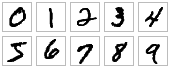 - -**The [MNIST dataset](http://yann.lecun.com/exdb/mnist/) comprises 60,000 -training examples and 10,000 test examples of the handwritten digits 0–9, -formatted as 28x28-pixel monochrome images.** - -## Getting Started - -Let's set up the skeleton for our TensorFlow program. Create a file called -`cnn_mnist.py`, and add the following code: - -```python -from __future__ import absolute_import -from __future__ import division -from __future__ import print_function - -# Imports -import numpy as np -import tensorflow as tf - -tf.logging.set_verbosity(tf.logging.INFO) - -# Our application logic will be added here - -if __name__ == "__main__": - tf.app.run() -``` - -As you work through the tutorial, you'll add code to construct, train, and -evaluate the convolutional neural network. The complete, final code can be -[found here](https://www.tensorflow.org/code/tensorflow/examples/tutorials/layers/cnn_mnist.py). - -## Intro to Convolutional Neural Networks - -Convolutional neural networks (CNNs) are the current state-of-the-art model -architecture for image classification tasks. CNNs apply a series of filters to -the raw pixel data of an image to extract and learn higher-level features, which -the model can then use for classification. CNNs contains three components: - -* **Convolutional layers**, which apply a specified number of convolution - filters to the image. For each subregion, the layer performs a set of - mathematical operations to produce a single value in the output feature map. - Convolutional layers then typically apply a - [ReLU activation function](https://en.wikipedia.org/wiki/Rectifier_\(neural_networks\)) to - the output to introduce nonlinearities into the model. - -* **Pooling layers**, which - [downsample the image data](https://en.wikipedia.org/wiki/Convolutional_neural_network#Pooling_layer) - extracted by the convolutional layers to reduce the dimensionality of the - feature map in order to decrease processing time. A commonly used pooling - algorithm is max pooling, which extracts subregions of the feature map - (e.g., 2x2-pixel tiles), keeps their maximum value, and discards all other - values. - -* **Dense (fully connected) layers**, which perform classification on the - features extracted by the convolutional layers and downsampled by the - pooling layers. In a dense layer, every node in the layer is connected to - every node in the preceding layer. - -Typically, a CNN is composed of a stack of convolutional modules that perform -feature extraction. Each module consists of a convolutional layer followed by a -pooling layer. The last convolutional module is followed by one or more dense -layers that perform classification. The final dense layer in a CNN contains a -single node for each target class in the model (all the possible classes the -model may predict), with a -[softmax](https://en.wikipedia.org/wiki/Softmax_function) activation function to -generate a value between 0–1 for each node (the sum of all these softmax values -is equal to 1). We can interpret the softmax values for a given image as -relative measurements of how likely it is that the image falls into each target -class. - -> Note: For a more comprehensive walkthrough of CNN architecture, see Stanford -> University's <a href="https://cs231n.github.io/convolutional-networks/"> -> Convolutional Neural Networks for Visual Recognition course materials</a>.</p> - -## Building the CNN MNIST Classifier {#building_the_cnn_mnist_classifier} - -Let's build a model to classify the images in the MNIST dataset using the -following CNN architecture: - -1. **Convolutional Layer #1**: Applies 32 5x5 filters (extracting 5x5-pixel - subregions), with ReLU activation function -2. **Pooling Layer #1**: Performs max pooling with a 2x2 filter and stride of 2 - (which specifies that pooled regions do not overlap) -3. **Convolutional Layer #2**: Applies 64 5x5 filters, with ReLU activation - function -4. **Pooling Layer #2**: Again, performs max pooling with a 2x2 filter and - stride of 2 -5. **Dense Layer #1**: 1,024 neurons, with dropout regularization rate of 0.4 - (probability of 0.4 that any given element will be dropped during training) -6. **Dense Layer #2 (Logits Layer)**: 10 neurons, one for each digit target - class (0–9). - -The `tf.layers` module contains methods to create each of the three layer types -above: - -* `conv2d()`. Constructs a two-dimensional convolutional layer. Takes number - of filters, filter kernel size, padding, and activation function as - arguments. -* `max_pooling2d()`. Constructs a two-dimensional pooling layer using the - max-pooling algorithm. Takes pooling filter size and stride as arguments. -* `dense()`. Constructs a dense layer. Takes number of neurons and activation - function as arguments. - -Each of these methods accepts a tensor as input and returns a transformed tensor -as output. This makes it easy to connect one layer to another: just take the -output from one layer-creation method and supply it as input to another. - -Open `cnn_mnist.py` and add the following `cnn_model_fn` function, which -conforms to the interface expected by TensorFlow's Estimator API (more on this -later in [Create the Estimator](#create-the-estimator)). `cnn_mnist.py` takes -MNIST feature data, labels, and mode (from -`tf.estimator.ModeKeys`: `TRAIN`, `EVAL`, `PREDICT`) as arguments; -configures the CNN; and returns predictions, loss, and a training operation: - -```python -def cnn_model_fn(features, labels, mode): - """Model function for CNN.""" - # Input Layer - input_layer = tf.reshape(features["x"], [-1, 28, 28, 1]) - - # Convolutional Layer #1 - conv1 = tf.layers.conv2d( - inputs=input_layer, - filters=32, - kernel_size=[5, 5], - padding="same", - activation=tf.nn.relu) - - # Pooling Layer #1 - pool1 = tf.layers.max_pooling2d(inputs=conv1, pool_size=[2, 2], strides=2) - - # Convolutional Layer #2 and Pooling Layer #2 - conv2 = tf.layers.conv2d( - inputs=pool1, - filters=64, - kernel_size=[5, 5], - padding="same", - activation=tf.nn.relu) - pool2 = tf.layers.max_pooling2d(inputs=conv2, pool_size=[2, 2], strides=2) - - # Dense Layer - pool2_flat = tf.reshape(pool2, [-1, 7 * 7 * 64]) - dense = tf.layers.dense(inputs=pool2_flat, units=1024, activation=tf.nn.relu) - dropout = tf.layers.dropout( - inputs=dense, rate=0.4, training=mode == tf.estimator.ModeKeys.TRAIN) - - # Logits Layer - logits = tf.layers.dense(inputs=dropout, units=10) - - predictions = { - # Generate predictions (for PREDICT and EVAL mode) - "classes": tf.argmax(input=logits, axis=1), - # Add `softmax_tensor` to the graph. It is used for PREDICT and by the - # `logging_hook`. - "probabilities": tf.nn.softmax(logits, name="softmax_tensor") - } - - if mode == tf.estimator.ModeKeys.PREDICT: - return tf.estimator.EstimatorSpec(mode=mode, predictions=predictions) - - # Calculate Loss (for both TRAIN and EVAL modes) - loss = tf.losses.sparse_softmax_cross_entropy(labels=labels, logits=logits) - - # Configure the Training Op (for TRAIN mode) - if mode == tf.estimator.ModeKeys.TRAIN: - optimizer = tf.train.GradientDescentOptimizer(learning_rate=0.001) - train_op = optimizer.minimize( - loss=loss, - global_step=tf.train.get_global_step()) - return tf.estimator.EstimatorSpec(mode=mode, loss=loss, train_op=train_op) - - # Add evaluation metrics (for EVAL mode) - eval_metric_ops = { - "accuracy": tf.metrics.accuracy( - labels=labels, predictions=predictions["classes"])} - return tf.estimator.EstimatorSpec( - mode=mode, loss=loss, eval_metric_ops=eval_metric_ops) -``` - -The following sections (with headings corresponding to each code block above) -dive deeper into the `tf.layers` code used to create each layer, as well as how -to calculate loss, configure the training op, and generate predictions. If -you're already experienced with CNNs and [TensorFlow `Estimator`s](../../guide/custom_estimators.md), -and find the above code intuitive, you may want to skim these sections or just -skip ahead to ["Training and Evaluating the CNN MNIST Classifier"](#train_eval_mnist). - -### Input Layer - -The methods in the `layers` module for creating convolutional and pooling layers -for two-dimensional image data expect input tensors to have a shape of -<code>[<em>batch_size</em>, <em>image_height</em>, <em>image_width</em>, -<em>channels</em>]</code> by default. This behavior can be changed using the <code><em>data_format</em></code> parameter; defined as follows: - - -* _`batch_size`_. Size of the subset of examples to use when performing - gradient descent during training. -* _`image_height`_. Height of the example images. -* _`image_width`_. Width of the example images. -* _`channels`_. Number of color channels in the example images. For color - images, the number of channels is 3 (red, green, blue). For monochrome - images, there is just 1 channel (black). -* _`data_format`_. A string, one of `channels_last` (default) or `channels_first`. - `channels_last` corresponds to inputs with shape - `(batch, ..., channels)` while `channels_first` corresponds to - inputs with shape `(batch, channels, ...)`. - -Here, our MNIST dataset is composed of monochrome 28x28 pixel images, so the -desired shape for our input layer is <code>[<em>batch_size</em>, 28, 28, -1]</code>. - -To convert our input feature map (`features`) to this shape, we can perform the -following `reshape` operation: - -```python -input_layer = tf.reshape(features["x"], [-1, 28, 28, 1]) -``` - -Note that we've indicated `-1` for batch size, which specifies that this -dimension should be dynamically computed based on the number of input values in -`features["x"]`, holding the size of all other dimensions constant. This allows -us to treat `batch_size` as a hyperparameter that we can tune. For example, if -we feed examples into our model in batches of 5, `features["x"]` will contain -3,920 values (one value for each pixel in each image), and `input_layer` will -have a shape of `[5, 28, 28, 1]`. Similarly, if we feed examples in batches of -100, `features["x"]` will contain 78,400 values, and `input_layer` will have a -shape of `[100, 28, 28, 1]`. - -### Convolutional Layer #1 - -In our first convolutional layer, we want to apply 32 5x5 filters to the input -layer, with a ReLU activation function. We can use the `conv2d()` method in the -`layers` module to create this layer as follows: - -```python -conv1 = tf.layers.conv2d( - inputs=input_layer, - filters=32, - kernel_size=[5, 5], - padding="same", - activation=tf.nn.relu) -``` - -The `inputs` argument specifies our input tensor, which must have the shape -<code>[<em>batch_size</em>, <em>image_height</em>, <em>image_width</em>, -<em>channels</em>]</code>. Here, we're connecting our first convolutional layer -to `input_layer`, which has the shape <code>[<em>batch_size</em>, 28, 28, -1]</code>. - -> Note: <code>conv2d()</code> will instead accept a shape of -> <code>[<em>batch_size</em>, <em>channels</em>, <em>image_height</em>, <em>image_width</em>]</code> when passed the argument -> <code>data_format=channels_first</code>. - -The `filters` argument specifies the number of filters to apply (here, 32), and -`kernel_size` specifies the dimensions of the filters as <code>[<em>height</em>, -<em>width</em>]</code> (here, <code>[5, 5]</code>). - -<p class="tip"><b>TIP:</b> If filter height and width have the same value, you can instead specify a -single integer for <code>kernel_size</code>—e.g., <code>kernel_size=5</code>.</p> - -The `padding` argument specifies one of two enumerated values -(case-insensitive): `valid` (default value) or `same`. To specify that the -output tensor should have the same height and width values as the input tensor, -we set `padding=same` here, which instructs TensorFlow to add 0 values to the -edges of the input tensor to preserve height and width of 28. (Without padding, -a 5x5 convolution over a 28x28 tensor will produce a 24x24 tensor, as there are -24x24 locations to extract a 5x5 tile from a 28x28 grid.) - -The `activation` argument specifies the activation function to apply to the -output of the convolution. Here, we specify ReLU activation with -`tf.nn.relu`. - -Our output tensor produced by `conv2d()` has a shape of -<code>[<em>batch_size</em>, 28, 28, 32]</code>: the same height and width -dimensions as the input, but now with 32 channels holding the output from each -of the filters. - -### Pooling Layer #1 - -Next, we connect our first pooling layer to the convolutional layer we just -created. We can use the `max_pooling2d()` method in `layers` to construct a -layer that performs max pooling with a 2x2 filter and stride of 2: - -```python -pool1 = tf.layers.max_pooling2d(inputs=conv1, pool_size=[2, 2], strides=2) -``` - -Again, `inputs` specifies the input tensor, with a shape of -<code>[<em>batch_size</em>, <em>image_height</em>, <em>image_width</em>, -<em>channels</em>]</code>. Here, our input tensor is `conv1`, the output from -the first convolutional layer, which has a shape of <code>[<em>batch_size</em>, -28, 28, 32]</code>. - -> Note: As with <code>conv2d()</code>, <code>max_pooling2d()</code> will instead -> accept a shape of <code>[<em>batch_size</em>, <em>channels</em>, -> <em>image_height</em>, <em>image_width</em>]</code> when passed the argument -> <code>data_format=channels_first</code>. - -The `pool_size` argument specifies the size of the max pooling filter as -<code>[<em>height</em>, <em>width</em>]</code> (here, `[2, 2]`). If both -dimensions have the same value, you can instead specify a single integer (e.g., -`pool_size=2`). - -The `strides` argument specifies the size of the stride. Here, we set a stride -of 2, which indicates that the subregions extracted by the filter should be -separated by 2 pixels in both the height and width dimensions (for a 2x2 filter, -this means that none of the regions extracted will overlap). If you want to set -different stride values for height and width, you can instead specify a tuple or -list (e.g., `stride=[3, 6]`). - -Our output tensor produced by `max_pooling2d()` (`pool1`) has a shape of -<code>[<em>batch_size</em>, 14, 14, 32]</code>: the 2x2 filter reduces height and width by 50% each. - -### Convolutional Layer #2 and Pooling Layer #2 - -We can connect a second convolutional and pooling layer to our CNN using -`conv2d()` and `max_pooling2d()` as before. For convolutional layer #2, we -configure 64 5x5 filters with ReLU activation, and for pooling layer #2, we use -the same specs as pooling layer #1 (a 2x2 max pooling filter with stride of 2): - -```python -conv2 = tf.layers.conv2d( - inputs=pool1, - filters=64, - kernel_size=[5, 5], - padding="same", - activation=tf.nn.relu) - -pool2 = tf.layers.max_pooling2d(inputs=conv2, pool_size=[2, 2], strides=2) -``` - -Note that convolutional layer #2 takes the output tensor of our first pooling -layer (`pool1`) as input, and produces the tensor `conv2` as output. `conv2` -has a shape of <code>[<em>batch_size</em>, 14, 14, 64]</code>, the same height and width as `pool1` (due to `padding="same"`), and 64 channels for the 64 -filters applied. - -Pooling layer #2 takes `conv2` as input, producing `pool2` as output. `pool2` -has shape <code>[<em>batch_size</em>, 7, 7, 64]</code> (50% reduction of height and width from `conv2`). - -### Dense Layer - -Next, we want to add a dense layer (with 1,024 neurons and ReLU activation) to -our CNN to perform classification on the features extracted by the -convolution/pooling layers. Before we connect the layer, however, we'll flatten -our feature map (`pool2`) to shape <code>[<em>batch_size</em>, -<em>features</em>]</code>, so that our tensor has only two dimensions: - -```python -pool2_flat = tf.reshape(pool2, [-1, 7 * 7 * 64]) -``` - -In the `reshape()` operation above, the `-1` signifies that the *`batch_size`* -dimension will be dynamically calculated based on the number of examples in our -input data. Each example has 7 (`pool2` height) * 7 (`pool2` width) * 64 -(`pool2` channels) features, so we want the `features` dimension to have a value -of 7 * 7 * 64 (3136 in total). The output tensor, `pool2_flat`, has shape -<code>[<em>batch_size</em>, 3136]</code>. - -Now, we can use the `dense()` method in `layers` to connect our dense layer as -follows: - -```python -dense = tf.layers.dense(inputs=pool2_flat, units=1024, activation=tf.nn.relu) -``` - -The `inputs` argument specifies the input tensor: our flattened feature map, -`pool2_flat`. The `units` argument specifies the number of neurons in the dense -layer (1,024). The `activation` argument takes the activation function; again, -we'll use `tf.nn.relu` to add ReLU activation. - -To help improve the results of our model, we also apply dropout regularization -to our dense layer, using the `dropout` method in `layers`: - -```python -dropout = tf.layers.dropout( - inputs=dense, rate=0.4, training=mode == tf.estimator.ModeKeys.TRAIN) -``` - -Again, `inputs` specifies the input tensor, which is the output tensor from our -dense layer (`dense`). - -The `rate` argument specifies the dropout rate; here, we use `0.4`, which means -40% of the elements will be randomly dropped out during training. - -The `training` argument takes a boolean specifying whether or not the model is -currently being run in training mode; dropout will only be performed if -`training` is `True`. Here, we check if the `mode` passed to our model function -`cnn_model_fn` is `TRAIN` mode. - -Our output tensor `dropout` has shape <code>[<em>batch_size</em>, 1024]</code>. - -### Logits Layer - -The final layer in our neural network is the logits layer, which will return the -raw values for our predictions. We create a dense layer with 10 neurons (one for -each target class 0–9), with linear activation (the default): - -```python -logits = tf.layers.dense(inputs=dropout, units=10) -``` - -Our final output tensor of the CNN, `logits`, has shape -<code>[<em>batch_size</em>, 10]</code>. - -### Generate Predictions {#generate_predictions} - -The logits layer of our model returns our predictions as raw values in a -<code>[<em>batch_size</em>, 10]</code>-dimensional tensor. Let's convert these -raw values into two different formats that our model function can return: - -* The **predicted class** for each example: a digit from 0–9. -* The **probabilities** for each possible target class for each example: the - probability that the example is a 0, is a 1, is a 2, etc. - -For a given example, our predicted class is the element in the corresponding row -of the logits tensor with the highest raw value. We can find the index of this -element using the `tf.argmax` -function: - -```python -tf.argmax(input=logits, axis=1) -``` - -The `input` argument specifies the tensor from which to extract maximum -values—here `logits`. The `axis` argument specifies the axis of the `input` -tensor along which to find the greatest value. Here, we want to find the largest -value along the dimension with index of 1, which corresponds to our predictions -(recall that our logits tensor has shape <code>[<em>batch_size</em>, -10]</code>). - -We can derive probabilities from our logits layer by applying softmax activation -using `tf.nn.softmax`: - -```python -tf.nn.softmax(logits, name="softmax_tensor") -``` - -> Note: We use the `name` argument to explicitly name this operation -> `softmax_tensor`, so we can reference it later. (We'll set up logging for the -> softmax values in ["Set Up a Logging Hook"](#set-up-a-logging-hook)). - -We compile our predictions in a dict, and return an `EstimatorSpec` object: - -```python -predictions = { - "classes": tf.argmax(input=logits, axis=1), - "probabilities": tf.nn.softmax(logits, name="softmax_tensor") -} -if mode == tf.estimator.ModeKeys.PREDICT: - return tf.estimator.EstimatorSpec(mode=mode, predictions=predictions) -``` - -### Calculate Loss {#calculating-loss} - -For both training and evaluation, we need to define a -[loss function](https://en.wikipedia.org/wiki/Loss_function) -that measures how closely the model's predictions match the target classes. For -multiclass classification problems like MNIST, -[cross entropy](https://en.wikipedia.org/wiki/Cross_entropy) is typically used -as the loss metric. The following code calculates cross entropy when the model -runs in either `TRAIN` or `EVAL` mode: - -```python -loss = tf.losses.sparse_softmax_cross_entropy(labels=labels, logits=logits) -``` - -Let's take a closer look at what's happening above. - -Our `labels` tensor contains a list of prediction indices for our examples, e.g. `[1, -9, ...]`. `logits` contains the linear outputs of our last layer. - -`tf.losses.sparse_softmax_cross_entropy`, calculates the softmax crossentropy -(aka: categorical crossentropy, negative log-likelihood) from these two inputs -in an efficient, numerically stable way. - - -### Configure the Training Op - -In the previous section, we defined loss for our CNN as the softmax -cross-entropy of the logits layer and our labels. Let's configure our model to -optimize this loss value during training. We'll use a learning rate of 0.001 and -[stochastic gradient descent](https://en.wikipedia.org/wiki/Stochastic_gradient_descent) -as the optimization algorithm: - -```python -if mode == tf.estimator.ModeKeys.TRAIN: - optimizer = tf.train.GradientDescentOptimizer(learning_rate=0.001) - train_op = optimizer.minimize( - loss=loss, - global_step=tf.train.get_global_step()) - return tf.estimator.EstimatorSpec(mode=mode, loss=loss, train_op=train_op) -``` - -> Note: For a more in-depth look at configuring training ops for Estimator model -> functions, see ["Defining the training op for the model"](../../guide/custom_estimators.md#defining-the-training-op-for-the-model) -> in the ["Creating Estimations in tf.estimator"](../../guide/custom_estimators.md) tutorial. - - -### Add evaluation metrics - -To add accuracy metric in our model, we define `eval_metric_ops` dict in EVAL -mode as follows: - -```python -eval_metric_ops = { - "accuracy": tf.metrics.accuracy( - labels=labels, predictions=predictions["classes"])} -return tf.estimator.EstimatorSpec( - mode=mode, loss=loss, eval_metric_ops=eval_metric_ops) -``` - -<a id="train_eval_mnist"></a> -## Training and Evaluating the CNN MNIST Classifier - -We've coded our MNIST CNN model function; now we're ready to train and evaluate -it. - -### Load Training and Test Data - -First, let's load our training and test data. Add a `main()` function to -`cnn_mnist.py` with the following code: - -```python -def main(unused_argv): - # Load training and eval data - mnist = tf.contrib.learn.datasets.load_dataset("mnist") - train_data = mnist.train.images # Returns np.array - train_labels = np.asarray(mnist.train.labels, dtype=np.int32) - eval_data = mnist.test.images # Returns np.array - eval_labels = np.asarray(mnist.test.labels, dtype=np.int32) -``` - -We store the training feature data (the raw pixel values for 55,000 images of -hand-drawn digits) and training labels (the corresponding value from 0–9 for -each image) as [numpy -arrays](https://docs.scipy.org/doc/numpy/reference/generated/numpy.array.html) -in `train_data` and `train_labels`, respectively. Similarly, we store the -evaluation feature data (10,000 images) and evaluation labels in `eval_data` -and `eval_labels`, respectively. - -### Create the Estimator {#create-the-estimator} - -Next, let's create an `Estimator` (a TensorFlow class for performing high-level -model training, evaluation, and inference) for our model. Add the following code -to `main()`: - -```python -# Create the Estimator -mnist_classifier = tf.estimator.Estimator( - model_fn=cnn_model_fn, model_dir="/tmp/mnist_convnet_model") -``` - -The `model_fn` argument specifies the model function to use for training, -evaluation, and prediction; we pass it the `cnn_model_fn` we created in -["Building the CNN MNIST Classifier."](#building-the-cnn-mnist-classifier) The -`model_dir` argument specifies the directory where model data (checkpoints) will -be saved (here, we specify the temp directory `/tmp/mnist_convnet_model`, but -feel free to change to another directory of your choice). - -> Note: For an in-depth walkthrough of the TensorFlow `Estimator` API, see the -> tutorial ["Creating Estimators in tf.estimator."](../../guide/custom_estimators.md) - -### Set Up a Logging Hook {#set_up_a_logging_hook} - -Since CNNs can take a while to train, let's set up some logging so we can track -progress during training. We can use TensorFlow's `tf.train.SessionRunHook` to create a -`tf.train.LoggingTensorHook` -that will log the probability values from the softmax layer of our CNN. Add the -following to `main()`: - -```python -# Set up logging for predictions -tensors_to_log = {"probabilities": "softmax_tensor"} -logging_hook = tf.train.LoggingTensorHook( - tensors=tensors_to_log, every_n_iter=50) -``` - -We store a dict of the tensors we want to log in `tensors_to_log`. Each key is a -label of our choice that will be printed in the log output, and the -corresponding label is the name of a `Tensor` in the TensorFlow graph. Here, our -`probabilities` can be found in `softmax_tensor`, the name we gave our softmax -operation earlier when we generated the probabilities in `cnn_model_fn`. - -> Note: If you don't explicitly assign a name to an operation via the `name` -> argument, TensorFlow will assign a default name. A couple easy ways to -> discover the names applied to operations are to visualize your graph on -> [TensorBoard](../../guide/graph_viz.md)) or to enable the -> [TensorFlow Debugger (tfdbg)](../../guide/debugger.md). - -Next, we create the `LoggingTensorHook`, passing `tensors_to_log` to the -`tensors` argument. We set `every_n_iter=50`, which specifies that probabilities -should be logged after every 50 steps of training. - -### Train the Model - -Now we're ready to train our model, which we can do by creating `train_input_fn` -and calling `train()` on `mnist_classifier`. Add the following to `main()`: - -```python -# Train the model -train_input_fn = tf.estimator.inputs.numpy_input_fn( - x={"x": train_data}, - y=train_labels, - batch_size=100, - num_epochs=None, - shuffle=True) -mnist_classifier.train( - input_fn=train_input_fn, - steps=20000, - hooks=[logging_hook]) -``` - -In the `numpy_input_fn` call, we pass the training feature data and labels to -`x` (as a dict) and `y`, respectively. We set a `batch_size` of `100` (which -means that the model will train on minibatches of 100 examples at each step). -`num_epochs=None` means that the model will train until the specified number of -steps is reached. We also set `shuffle=True` to shuffle the training data. -In the `train` call, we set `steps=20000` -(which means the model will train for 20,000 steps total). We pass our -`logging_hook` to the `hooks` argument, so that it will be triggered during -training. - -### Evaluate the Model - -Once training is complete, we want to evaluate our model to determine its -accuracy on the MNIST test set. We call the `evaluate` method, which evaluates -the metrics we specified in `eval_metric_ops` argument in the `model_fn`. -Add the following to `main()`: - -```python -# Evaluate the model and print results -eval_input_fn = tf.estimator.inputs.numpy_input_fn( - x={"x": eval_data}, - y=eval_labels, - num_epochs=1, - shuffle=False) -eval_results = mnist_classifier.evaluate(input_fn=eval_input_fn) -print(eval_results) -``` - -To create `eval_input_fn`, we set `num_epochs=1`, so that the model evaluates -the metrics over one epoch of data and returns the result. We also set -`shuffle=False` to iterate through the data sequentially. - -### Run the Model - -We've coded the CNN model function, `Estimator`, and the training/evaluation -logic; now let's see the results. Run `cnn_mnist.py`. - -> Note: Training CNNs is quite computationally intensive. Estimated completion -> time of `cnn_mnist.py` will vary depending on your processor, but will likely -> be upwards of 1 hour on CPU. To train more quickly, you can decrease the -> number of `steps` passed to `train()`, but note that this will affect accuracy. - -As the model trains, you'll see log output like the following: - -```python -INFO:tensorflow:loss = 2.36026, step = 1 -INFO:tensorflow:probabilities = [[ 0.07722801 0.08618255 0.09256398, ...]] -... -INFO:tensorflow:loss = 2.13119, step = 101 -INFO:tensorflow:global_step/sec: 5.44132 -... -INFO:tensorflow:Loss for final step: 0.553216. - -INFO:tensorflow:Restored model from /tmp/mnist_convnet_model -INFO:tensorflow:Eval steps [0,inf) for training step 20000. -INFO:tensorflow:Input iterator is exhausted. -INFO:tensorflow:Saving evaluation summary for step 20000: accuracy = 0.9733, loss = 0.0902271 -{'loss': 0.090227105, 'global_step': 20000, 'accuracy': 0.97329998} -``` - -Here, we've achieved an accuracy of 97.3% on our test data set. - -## Additional Resources - -To learn more about TensorFlow Estimators and CNNs in TensorFlow, see the -following resources: - -* [Creating Estimators in tf.estimator](../../guide/custom_estimators.md) - provides an introduction to the TensorFlow Estimator API. It walks through - configuring an Estimator, writing a model function, calculating loss, and - defining a training op. -* [Advanced Convolutional Neural Networks](../../tutorials/images/deep_cnn.md) walks through how to build a MNIST CNN classification model - *without estimators* using lower-level TensorFlow operations. |