
diff options
Diffstat (limited to 'tensorflow/docs_src/guide/low_level_intro.md')
| -rw-r--r-- | tensorflow/docs_src/guide/low_level_intro.md | 604 |
1 files changed, 0 insertions, 604 deletions
diff --git a/tensorflow/docs_src/guide/low_level_intro.md b/tensorflow/docs_src/guide/low_level_intro.md deleted file mode 100644 index d002f8af0b..0000000000 --- a/tensorflow/docs_src/guide/low_level_intro.md +++ /dev/null @@ -1,604 +0,0 @@ -# Introduction - -This guide gets you started programming in the low-level TensorFlow APIs -(TensorFlow Core), showing you how to: - - * Manage your own TensorFlow program (a `tf.Graph`) and TensorFlow - runtime (a `tf.Session`), instead of relying on Estimators to manage them. - * Run TensorFlow operations, using a `tf.Session`. - * Use high level components ([datasets](#datasets), [layers](#layers), and - [feature_columns](#feature_columns)) in this low level environment. - * Build your own training loop, instead of using the one - [provided by Estimators](../guide/premade_estimators.md). - -We recommend using the higher level APIs to build models when possible. -Knowing TensorFlow Core is valuable for the following reasons: - - * Experimentation and debugging are both more straight forward - when you can use low level TensorFlow operations directly. - * It gives you a mental model of how things work internally when - using the higher level APIs. - -## Setup - -Before using this guide, [install TensorFlow](../install/index.md). - -To get the most out of this guide, you should know the following: - -* How to program in Python. -* At least a little bit about arrays. -* Ideally, something about machine learning. - -Feel free to launch `python` and follow along with this walkthrough. -Run the following lines to set up your Python environment: - -```python -from __future__ import absolute_import -from __future__ import division -from __future__ import print_function - -import numpy as np -import tensorflow as tf -``` - -## Tensor Values - -The central unit of data in TensorFlow is the **tensor**. A tensor consists of a -set of primitive values shaped into an array of any number of dimensions. A -tensor's **rank** is its number of dimensions, while its **shape** is a tuple -of integers specifying the array's length along each dimension. Here are some -examples of tensor values: - -```python -3. # a rank 0 tensor; a scalar with shape [], -[1., 2., 3.] # a rank 1 tensor; a vector with shape [3] -[[1., 2., 3.], [4., 5., 6.]] # a rank 2 tensor; a matrix with shape [2, 3] -[[[1., 2., 3.]], [[7., 8., 9.]]] # a rank 3 tensor with shape [2, 1, 3] -``` - -TensorFlow uses numpy arrays to represent tensor **values**. - -## TensorFlow Core Walkthrough - -You might think of TensorFlow Core programs as consisting of two discrete -sections: - -1. Building the computational graph (a `tf.Graph`). -2. Running the computational graph (using a `tf.Session`). - -### Graph - -A **computational graph** is a series of TensorFlow operations arranged into a -graph. The graph is composed of two types of objects. - - * `tf.Operation` (or "ops"): The nodes of the graph. - Operations describe calculations that consume and produce tensors. - * `tf.Tensor`: The edges in the graph. These represent the values - that will flow through the graph. Most TensorFlow functions return - `tf.Tensors`. - -Important: `tf.Tensors` do not have values, they are just handles to elements -in the computation graph. - -Let's build a simple computational graph. The most basic operation is a -constant. The Python function that builds the operation takes a tensor value as -input. The resulting operation takes no inputs. When run, it outputs the -value that was passed to the constructor. We can create two floating point -constants `a` and `b` as follows: - -```python -a = tf.constant(3.0, dtype=tf.float32) -b = tf.constant(4.0) # also tf.float32 implicitly -total = a + b -print(a) -print(b) -print(total) -``` - -The print statements produce: - -``` -Tensor("Const:0", shape=(), dtype=float32) -Tensor("Const_1:0", shape=(), dtype=float32) -Tensor("add:0", shape=(), dtype=float32) -``` - -Notice that printing the tensors does not output the values `3.0`, `4.0`, and -`7.0` as you might expect. The above statements only build the computation -graph. These `tf.Tensor` objects just represent the results of the operations -that will be run. - -Each operation in a graph is given a unique name. This name is independent of -the names the objects are assigned to in Python. Tensors are named after the -operation that produces them followed by an output index, as in -`"add:0"` above. - -### TensorBoard - -TensorFlow provides a utility called TensorBoard. One of TensorBoard's many -capabilities is visualizing a computation graph. You can easily do this with -a few simple commands. - -First you save the computation graph to a TensorBoard summary file as -follows: - -``` -writer = tf.summary.FileWriter('.') -writer.add_graph(tf.get_default_graph()) -``` - -This will produce an `event` file in the current directory with a name in the -following format: - -``` -events.out.tfevents.{timestamp}.{hostname} -``` - -Now, in a new terminal, launch TensorBoard with the following shell command: - -```bsh -tensorboard --logdir . -``` - -Then open TensorBoard's [graphs page](http://localhost:6006/#graphs) in your -browser, and you should see a graph similar to the following: - -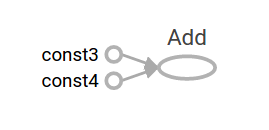 - -For more about TensorBoard's graph visualization tools see [TensorBoard: Graph Visualization](../guide/graph_viz.md). - -### Session - -To evaluate tensors, instantiate a `tf.Session` object, informally known as a -**session**. A session encapsulates the state of the TensorFlow runtime, and -runs TensorFlow operations. If a `tf.Graph` is like a `.py` file, a `tf.Session` -is like the `python` executable. - -The following code creates a `tf.Session` object and then invokes its `run` -method to evaluate the `total` tensor we created above: - -```python -sess = tf.Session() -print(sess.run(total)) -``` - -When you request the output of a node with `Session.run` TensorFlow backtracks -through the graph and runs all the nodes that provide input to the requested -output node. So this prints the expected value of 7.0: - -``` -7.0 -``` - -You can pass multiple tensors to `tf.Session.run`. The `run` method -transparently handles any combination of tuples or dictionaries, as in the -following example: - -```python -print(sess.run({'ab':(a, b), 'total':total})) -``` - -which returns the results in a structure of the same layout: - -``` None -{'total': 7.0, 'ab': (3.0, 4.0)} -``` - -During a call to `tf.Session.run` any `tf.Tensor` only has a single value. -For example, the following code calls `tf.random_uniform` to produce a -`tf.Tensor` that generates a random 3-element vector (with values in `[0,1)`): - -```python -vec = tf.random_uniform(shape=(3,)) -out1 = vec + 1 -out2 = vec + 2 -print(sess.run(vec)) -print(sess.run(vec)) -print(sess.run((out1, out2))) -``` - -The result shows a different random value on each call to `run`, but -a consistent value during a single `run` (`out1` and `out2` receive the same -random input): - -``` -[ 0.52917576 0.64076328 0.68353939] -[ 0.66192627 0.89126778 0.06254101] -( - array([ 1.88408756, 1.87149239, 1.84057522], dtype=float32), - array([ 2.88408756, 2.87149239, 2.84057522], dtype=float32) -) -``` - -Some TensorFlow functions return `tf.Operations` instead of `tf.Tensors`. -The result of calling `run` on an Operation is `None`. You run an operation -to cause a side-effect, not to retrieve a value. Examples of this include the -[initialization](#Initializing Layers), and [training](#Training) ops -demonstrated later. - -### Feeding - -As it stands, this graph is not especially interesting because it always -produces a constant result. A graph can be parameterized to accept external -inputs, known as **placeholders**. A **placeholder** is a promise to provide a -value later, like a function argument. - -```python -x = tf.placeholder(tf.float32) -y = tf.placeholder(tf.float32) -z = x + y -``` - -The preceding three lines are a bit like a function in which we -define two input parameters (`x` and `y`) and then an operation on them. We can -evaluate this graph with multiple inputs by using the `feed_dict` argument of -the `tf.Session.run` method to feed concrete values to the placeholders: - -```python -print(sess.run(z, feed_dict={x: 3, y: 4.5})) -print(sess.run(z, feed_dict={x: [1, 3], y: [2, 4]})) -``` -This results in the following output: - -``` -7.5 -[ 3. 7.] -``` - -Also note that the `feed_dict` argument can be used to overwrite any tensor in -the graph. The only difference between placeholders and other `tf.Tensors` is -that placeholders throw an error if no value is fed to them. - -## Datasets - -Placeholders work for simple experiments, but `tf.data` are the -preferred method of streaming data into a model. - -To get a runnable `tf.Tensor` from a Dataset you must first convert it to a -`tf.data.Iterator`, and then call the Iterator's -`tf.data.Iterator.get_next` method. - -The simplest way to create an Iterator is with the -`tf.data.Dataset.make_one_shot_iterator` method. -For example, in the following code the `next_item` tensor will return a row from -the `my_data` array on each `run` call: - -``` python -my_data = [ - [0, 1,], - [2, 3,], - [4, 5,], - [6, 7,], -] -slices = tf.data.Dataset.from_tensor_slices(my_data) -next_item = slices.make_one_shot_iterator().get_next() -``` - -Reaching the end of the data stream causes `Dataset` to throw an -`tf.errors.OutOfRangeError`. For example, the following code -reads the `next_item` until there is no more data to read: - -``` python -while True: - try: - print(sess.run(next_item)) - except tf.errors.OutOfRangeError: - break -``` - -If the `Dataset` depends on stateful operations you may need to -initialize the iterator before using it, as shown below: - -``` python -r = tf.random_normal([10,3]) -dataset = tf.data.Dataset.from_tensor_slices(r) -iterator = dataset.make_initializable_iterator() -next_row = iterator.get_next() - -sess.run(iterator.initializer) -while True: - try: - print(sess.run(next_row)) - except tf.errors.OutOfRangeError: - break -``` - -For more details on Datasets and Iterators see: [Importing Data](../guide/datasets.md). - -## Layers - -A trainable model must modify the values in the graph to get new outputs with -the same input. `tf.layers` are the preferred way to add trainable -parameters to a graph. - -Layers package together both the variables and the operations that act -on them. For example a -[densely-connected layer](https://developers.google.com/machine-learning/glossary/#fully_connected_layer) -performs a weighted sum across all inputs -for each output and applies an optional -[activation function](https://developers.google.com/machine-learning/glossary/#activation_function). -The connection weights and biases are managed by the layer object. - -### Creating Layers - -The following code creates a `tf.layers.Dense` layer that takes a -batch of input vectors, and produces a single output value for each. To apply a -layer to an input, call the layer as if it were a function. For example: - -```python -x = tf.placeholder(tf.float32, shape=[None, 3]) -linear_model = tf.layers.Dense(units=1) -y = linear_model(x) -``` - -The layer inspects its input to determine sizes for its internal variables. So -here we must set the shape of the `x` placeholder so that the layer can -build a weight matrix of the correct size. - -Now that we have defined the calculation of the output, `y`, there is one more -detail we need to take care of before we run the calculation. - -### Initializing Layers - -The layer contains variables that must be **initialized** before they can be -used. While it is possible to initialize variables individually, you can easily -initialize all the variables in a TensorFlow graph as follows: - -```python -init = tf.global_variables_initializer() -sess.run(init) -``` - -Important: Calling `tf.global_variables_initializer` only -creates and returns a handle to a TensorFlow operation. That op -will initialize all the global variables when we run it with `tf.Session.run`. - -Also note that this `global_variables_initializer` only initializes variables -that existed in the graph when the initializer was created. So the initializer -should be one of the last things added during graph construction. - -### Executing Layers - -Now that the layer is initialized, we can evaluate the `linear_model`'s output -tensor as we would any other tensor. For example, the following code: - -```python -print(sess.run(y, {x: [[1, 2, 3],[4, 5, 6]]})) -``` - -will generate a two-element output vector such as the following: - -``` -[[-3.41378999] - [-9.14999008]] -``` - -### Layer Function shortcuts - -For each layer class (like `tf.layers.Dense`) TensorFlow also supplies a -shortcut function (like `tf.layers.dense`). The only difference is that the -shortcut function versions create and run the layer in a single call. For -example, the following code is equivalent to the earlier version: - -```python -x = tf.placeholder(tf.float32, shape=[None, 3]) -y = tf.layers.dense(x, units=1) - -init = tf.global_variables_initializer() -sess.run(init) - -print(sess.run(y, {x: [[1, 2, 3], [4, 5, 6]]})) -``` - -While convenient, this approach allows no access to the `tf.layers.Layer` -object. This makes introspection and debugging more difficult, -and layer reuse impossible. - -## Feature columns - -The easiest way to experiment with feature columns is using the -`tf.feature_column.input_layer` function. This function only accepts -[dense columns](../guide/feature_columns.md) as inputs, so to view the result -of a categorical column you must wrap it in an -`tf.feature_column.indicator_column`. For example: - -``` python -features = { - 'sales' : [[5], [10], [8], [9]], - 'department': ['sports', 'sports', 'gardening', 'gardening']} - -department_column = tf.feature_column.categorical_column_with_vocabulary_list( - 'department', ['sports', 'gardening']) -department_column = tf.feature_column.indicator_column(department_column) - -columns = [ - tf.feature_column.numeric_column('sales'), - department_column -] - -inputs = tf.feature_column.input_layer(features, columns) -``` - -Running the `inputs` tensor will parse the `features` into a batch of vectors. - -Feature columns can have internal state, like layers, so they often need to be -initialized. Categorical columns use `tf.contrib.lookup` -internally and these require a separate initialization op, -`tf.tables_initializer`. - -``` python -var_init = tf.global_variables_initializer() -table_init = tf.tables_initializer() -sess = tf.Session() -sess.run((var_init, table_init)) -``` - -Once the internal state has been initialized you can run `inputs` like any -other `tf.Tensor`: - -```python -print(sess.run(inputs)) -``` - -This shows how the feature columns have packed the input vectors, with the -one-hot "department" as the first two indices and "sales" as the third. - -```None -[[ 1. 0. 5.] - [ 1. 0. 10.] - [ 0. 1. 8.] - [ 0. 1. 9.]] -``` - -## Training - -Now that you're familiar with the basics of core TensorFlow, let's train a -small regression model manually. - -### Define the data - -First let's define some inputs, `x`, and the expected output for each input, -`y_true`: - -```python -x = tf.constant([[1], [2], [3], [4]], dtype=tf.float32) -y_true = tf.constant([[0], [-1], [-2], [-3]], dtype=tf.float32) -``` - -### Define the model - -Next, build a simple linear model, with 1 output: - -``` python -linear_model = tf.layers.Dense(units=1) - -y_pred = linear_model(x) -``` - -You can evaluate the predictions as follows: - -``` python -sess = tf.Session() -init = tf.global_variables_initializer() -sess.run(init) - -print(sess.run(y_pred)) -``` - -The model hasn't yet been trained, so the four "predicted" values aren't very -good. Here's what we got; your own output will almost certainly differ: - -``` None -[[ 0.02631879] - [ 0.05263758] - [ 0.07895637] - [ 0.10527515]] -``` - -### Loss - -To optimize a model, you first need to define the loss. We'll use the mean -square error, a standard loss for regression problems. - -While you could do this manually with lower level math operations, -the `tf.losses` module provides a set of common loss functions. You can use it -to calculate the mean square error as follows: - -``` python -loss = tf.losses.mean_squared_error(labels=y_true, predictions=y_pred) - -print(sess.run(loss)) -``` -This will produce a loss value, something like: - -``` None -2.23962 -``` - -### Training - -TensorFlow provides -[**optimizers**](https://developers.google.com/machine-learning/glossary/#optimizer) -implementing standard optimization algorithms. These are implemented as -sub-classes of `tf.train.Optimizer`. They incrementally change each -variable in order to minimize the loss. The simplest optimization algorithm is -[**gradient descent**](https://developers.google.com/machine-learning/glossary/#gradient_descent), -implemented by `tf.train.GradientDescentOptimizer`. It modifies each -variable according to the magnitude of the derivative of loss with respect to -that variable. For example: - -```python -optimizer = tf.train.GradientDescentOptimizer(0.01) -train = optimizer.minimize(loss) -``` - -This code builds all the graph components necessary for the optimization, and -returns a training operation. When run, the training op will update variables -in the graph. You might run it as follows: - -```python -for i in range(100): - _, loss_value = sess.run((train, loss)) - print(loss_value) -``` - -Since `train` is an op, not a tensor, it doesn't return a value when run. -To see the progression of the loss during training, we run the loss tensor at -the same time, producing output like the following: - -``` None -1.35659 -1.00412 -0.759167 -0.588829 -0.470264 -0.387626 -0.329918 -0.289511 -0.261112 -0.241046 -... -``` - -### Complete program - -```python -x = tf.constant([[1], [2], [3], [4]], dtype=tf.float32) -y_true = tf.constant([[0], [-1], [-2], [-3]], dtype=tf.float32) - -linear_model = tf.layers.Dense(units=1) - -y_pred = linear_model(x) -loss = tf.losses.mean_squared_error(labels=y_true, predictions=y_pred) - -optimizer = tf.train.GradientDescentOptimizer(0.01) -train = optimizer.minimize(loss) - -init = tf.global_variables_initializer() - -sess = tf.Session() -sess.run(init) -for i in range(100): - _, loss_value = sess.run((train, loss)) - print(loss_value) - -print(sess.run(y_pred)) -``` - -## Next steps - -To learn more about building models with TensorFlow consider the following: - -* [Custom Estimators](../guide/custom_estimators.md), to learn how to build - customized models with TensorFlow. Your knowledge of TensorFlow Core will - help you understand and debug your own models. - -If you want to learn more about the inner workings of TensorFlow consider the -following documents, which go into more depth on many of the topics discussed -here: - -* [Graphs and Sessions](../guide/graphs.md) -* [Tensors](../guide/tensors.md) -* [Variables](../guide/variables.md) - - |