path: root/tensorflow/docs_src/tutorials/image_retraining.md

# How to Retrain Inception's Final Layer for New Categories

Modern object recognition models have millions of parameters and can take weeks
to fully train. Transfer learning is a technique that shortcuts a lot of this
work by taking a fully-trained model for a set of categories like ImageNet, and
retrains from the existing weights for new classes. In this example we'll be
retraining the final layer from scratch, while leaving all the others untouched.
For more information on the approach you can see
[this paper on Decaf](http://arxiv.org/pdf/1310.1531v1.pdf).

Though it's not as good as a full training run, this is surprisingly effective
for many applications, and can be run in as little as thirty minutes on a
laptop, without requiring a GPU. This tutorial will show you how to run the
example script on your own images, and will explain some of the options you have
to help control the training process.

Note: This version of the tutorial mainly uses bazel. A bazel free version is
also available
[as a codelab](https://codelabs.developers.google.com/codelabs/tensorflow-for-poets/#0).

[TOC]

## Training on Flowers

![Daisies by Kelly Sikkema](https://www.tensorflow.org/images/daisies.jpg)

[Image by Kelly Sikkema](https://www.flickr.com/photos/95072945@N05/9922116524/)

Before you start any training, you'll need a set of images to teach the network
about the new classes you want to recognize. There's a later section that
explains how to prepare your own images, but to make it easy we've created an
archive of creative-commons licensed flower photos to use initially. To get the
set of flower photos, run these commands:

```sh
cd ~
curl -O http://download.tensorflow.org/example_images/flower_photos.tgz
tar xzf flower_photos.tgz
```

Once you have the images, you can build the retrainer like this, from the root
of your TensorFlow source directory:

```sh
bazel build tensorflow/examples/image_retraining:retrain
```

If you have a machine which supports
[the AVX instruction set](https://en.wikipedia.org/wiki/Advanced_Vector_Extensions)
(common in x86 CPUs produced in the last few years) you can improve the running
speed of the retraining by building for that architecture, like this (after choosing appropriate options in `configure`):

```sh
bazel build --config opt tensorflow/examples/image_retraining:retrain
```

The retrainer can then be run like this:

```sh
bazel-bin/tensorflow/examples/image_retraining/retrain --image_dir ~/flower_photos
```

This script loads the pre-trained Inception v3 model, removes the old top layer,
and trains a new one on the flower photos you've downloaded. None of the flower
species were in the original ImageNet classes the full network was trained on.
The magic of transfer learning is that lower layers that have been trained to
distinguish between some objects can be reused for many recognition tasks
without any alteration.

## Bottlenecks

The script can take thirty minutes or more to complete, depending on the speed
of your machine. The first phase analyzes all the images on disk and calculates
the bottleneck values for each of them. 'Bottleneck' is an informal term we
often use for the layer just before the final output layer that actually does
the classification. This penultimate layer has been trained to output a set of
values that's good enough for the classifier to use to distinguish between all
the classes it's been asked to recognize. That means it has to be a meaningful
and compact summary of the images, since it has to contain enough information
for the classifier to make a good choice in a very small set of values. The
reason our final layer retraining can work on new classes is that it turns out
the kind of information needed to distinguish between all the 1,000 classes in
ImageNet is often also useful to distinguish between new kinds of objects.

Because every image is reused multiple times during training and calculating
each bottleneck takes a significant amount of time, it speeds things up to
cache these bottleneck values on disk so they don't have to be repeatedly
recalculated. By default they're stored in the `/tmp/bottleneck` directory, and
if you rerun the script they'll be reused so you don't have to wait for this
part again.

## Training

Once the bottlenecks are complete, the actual training of the top layer of the
network begins. You'll see a series of step outputs, each one showing training
accuracy, validation accuracy, and the cross entropy. The training accuracy
shows what percent of the images used in the current training batch were
labeled with the correct class. The validation accuracy is the precision on a
randomly-selected group of images from a different set. The key difference is
that the training accuracy is based on images that the network has been able
to learn from so the network can overfit to the noise in the training data. A
true measure of the performance of the network is to measure its performance on
a data set not contained in the training data -- this is measured by the
validation accuracy. If the train accuracy is high but the validation accuracy
remains low, that means the network is overfitting and memorizing particular
features in the training images that aren't helpful more generally. Cross
entropy is a loss function which gives a glimpse into how well the learning
process is progressing. The training's objective is to make the loss as small as
possible, so you can tell if the learning is working by keeping an eye on
whether the loss keeps trending downwards, ignoring the short-term noise.

By default this script will run 4,000 training steps. Each step chooses ten
images at random from the training set, finds their bottlenecks from the cache,
and feeds them into the final layer to get predictions. Those predictions are
then compared against the actual labels to update the final layer's weights
through the back-propagation process. As the process continues you should see
the reported accuracy improve, and after all the steps are done, a final test
accuracy evaluation is run on a set of images kept separate from the training
and validation pictures. This test evaluation is the best estimate of how the
trained model will perform on the classification task. You should see an
accuracy value of between 90% and 95%, though the exact value will vary from run
to run since there's randomness in the training process. This number is based on
the percent of the images in the test set that are given the correct label
after the model is fully trained.

## Visualizing the Retraining with TensorBoard

The script includes TensorBoard summaries that make it easier to understand, debug, and optimize the retraining. For example, you can visualize the graph and statistics, such as how the weights or accuracy varied during training.

To launch TensorBoard, run this command during or after retraining:

```sh
tensorboard --logdir /tmp/retrain_logs
```

Once TensorBoard is running, navigate your web browser to `localhost:6006` to view the TensorBoard.

The script will log TensorBoard summaries to `/tmp/retrain_logs` by default. You can change the directory with the `--summaries_dir` flag.

The [TensorBoard's GitHub](https://github.com/tensorflow/tensorboard) has a lot more information on TensorBoard usage, including tips & tricks, and debugging information.

## Using the Retrained Model

The script will write out a version of the Inception v3 network with a final
layer retrained to your categories to /tmp/output_graph.pb, and a text file
containing the labels to /tmp/output_labels.txt. These are both in a format that
the @{$image_recognition$C++ and Python image classification examples}
can read in, so you can start using your new model immediately. Since you've
replaced the top layer, you will need to specify the new name in the script, for
example with the flag `--output_layer=final_result` if you're using label_image.

Here's an example of how to build and run the label_image example with your
retrained graphs:

```sh
bazel build tensorflow/examples/image_retraining:label_image && \
bazel-bin/tensorflow/examples/image_retraining/label_image \
--graph=/tmp/output_graph.pb --labels=/tmp/output_labels.txt \
--output_layer=final_result:0 \
--image=$HOME/flower_photos/daisy/21652746_cc379e0eea_m.jpg
```

You should see a list of flower labels, in most cases with daisy on top
(though each retrained model may be slightly different). You can replace the
`--image` parameter with your own images to try those out, and use the C++ code
as a template to integrate with your own applications.

If you'd like to use the retrained model in your own Python program, then the
above
[`label_image` script](https://www.tensorflow.org/code/tensorflow/examples/image_retraining/label_image.py)
is a reasonable starting point.

If you find the default Inception v3 model is too large or slow for your
application, take a look at the [Other Model Architectures section](/tutorials/image_retraining#other_model_architectures)
below for options to speed up and slim down your network.

## Training on Your Own Categories

If you've managed to get the script working on the flower example images, you
can start looking at teaching it to recognize categories you care about instead.
In theory all you'll need to do is point it at a set of sub-folders, each named
after one of your categories and containing only images from that category. If
you do that and pass the root folder of the subdirectories as the argument to
`--image_dir`, the script should train just like it did for the flowers.

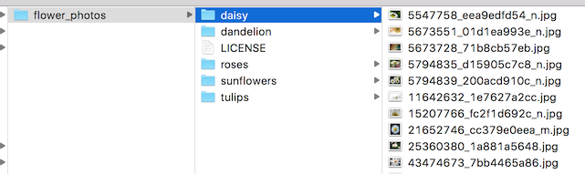
Here's what the folder structure of the flowers archive looks like, to give you
and example of the kind of layout the script is looking for:

![Folder Structure](https://www.tensorflow.org/images/folder_structure.png)

In practice it may take some work to get the accuracy you want. I'll try to
guide you through some of the common problems you might encounter below.

## Creating a Set of Training Images

The first place to start is by looking at the images you've gathered, since the
most common issues we see with training come from the data that's being fed in.

For training to work well, you should gather at least a hundred photos of each
kind of object you want to recognize. The more you can gather, the better the
accuracy of your trained model is likely to be. You also need to make sure that
the photos are a good representation of what your application will actually
encounter. For example, if you take all your photos indoors against a blank wall
and your users are trying to recognize objects outdoors, you probably won't see
good results when you deploy.

Another pitfall to avoid is that the learning process will pick up on anything
that the labeled images have in common with each other, and if you're not
careful that might be something that's not useful. For example if you photograph
one kind of object in a blue room, and another in a green one, then the model
will end up basing its prediction on the background color, not the features of
the object you actually care about. To avoid this, try to take pictures in as
wide a variety of situations as you can, at different times, and with different
devices. If you want to know more about this problem, you can read about the
classic (and possibly apocryphal)
[tank recognition problem](http://www.jefftk.com/p/detecting-tanks).

You may also want to think about the categories you use. It might be worth
splitting big categories that cover a lot of different physical forms into
smaller ones that are more visually distinct. For example instead of 'vehicle'
you might use 'car', 'motorbike', and 'truck'. It's also worth thinking about
whether you have a 'closed world' or an 'open world' problem. In a closed world,
the only things you'll ever be asked to categorize are the classes of object you
know about. This might apply to a plant recognition app where you know the user
is likely to be taking a picture of a flower, so all you have to do is decide
which species. By contrast a roaming robot might see all sorts of different
things through its camera as it wanders around the world. In that case you'd
want the classifier to report if it wasn't sure what it was seeing. This can be
hard to do well, but often if you collect a large number of typical 'background'
photos with no relevant objects in them, you can add them to an extra 'unknown'
class in your image folders.

It's also worth checking to make sure that all of your images are labeled
correctly. Often user-generated tags are unreliable for our purposes, for
example using #daisy for pictures of a person named Daisy. If you go through
your images and weed out any mistakes it can do wonders for your overall
accuracy.

## Training Steps

If you're happy with your images, you can take a look at improving your results
by altering the details of the learning process. The simplest one to try is
`--how_many_training_steps`. This defaults to 4,000, but if you increase it to
8,000 it will train for twice as long. The rate of improvement in the accuracy
slows the longer you train for, and at some point will stop altogether, but you
can experiment to see when you hit that limit for your model.

## Distortions

A common way of improving the results of image training is by deforming,
cropping, or brightening the training inputs in random ways. This has the
advantage of expanding the effective size of the training data thanks to all the
possible variations of the same images, and tends to help the network learn to
cope with all the distortions that will occur in real-life uses of the
classifier. The biggest disadvantage of enabling these distortions in our script
is that the bottleneck caching is no longer useful, since input images are never
reused exactly. This means the training process takes a lot longer, so I
recommend trying this as a way of fine-tuning your model once you've got one
that you're reasonably happy with.

You enable these distortions by passing `--random_crop`, `--random_scale` and
`--random_brightness` to the script. These are all percentage values that
control how much of each of the distortions is applied to each image. It's
reasonable to start with values of 5 or 10 for each of them and then experiment
to see which of them help with your application. `--flip_left_right` will
randomly mirror half of the images horizontally, which makes sense as long as
those inversions are likely to happen in your application. For example it
wouldn't be a good idea if you were trying to recognize letters, since flipping
them destroys their meaning.

## Hyper-parameters

There are several other parameters you can try adjusting to see if they help
your results. The `--learning_rate` controls the magnitude of the updates to the
final layer during training. Intuitively if this is smaller than the learning
will take longer, but it can end up helping the overall precision. That's not
always the case though, so you need to experiment carefully to see what works
for your case. The `--train_batch_size` controls how many images are examined
during one training step, and because the learning rate is applied per batch
you'll need to reduce it if you have larger batches to get the same overall
effect.

## Training, Validation, and Testing Sets

One of the things the script does under the hood when you point it at a folder
of images is divide them up into three different sets. The largest is usually
the training set, which are all the images fed into the network during training,
with the results used to update the model's weights. You might wonder why we
don't use all the images for training? A big potential problem when we're doing
machine learning is that our model may just be memorizing irrelevant details of
the training images to come up with the right answers. For example, you could
imagine a network remembering a pattern in the background of each photo it was
shown, and using that to match labels with objects. It could produce good
results on all the images it's seen before during training, but then fail on new
images because it's not learned general characteristics of the objects, just
memorized unimportant details of the training images.

This problem is known as overfitting, and to avoid it we keep some of our data
out of the training process, so that the model can't memorize them. We then use
those images as a check to make sure that overfitting isn't occurring, since if
we see good accuracy on them it's a good sign the network isn't overfitting. The
usual split is to put 80% of the images into the main training set, keep 10%
aside to run as validation frequently during training, and then have a final 10%
that are used less often as a testing set to predict the real-world performance
of the classifier. These ratios can be controlled using the
`--testing_percentage` and `--validation_percentage` flags. In general
you should be able to leave these values at their defaults, since you won't
usually find any advantage to training to adjusting them.

Note that the script uses the image filenames (rather than a completely random
function) to divide the images among the training, validation, and test sets.
This is done to ensure that images don't get moved between training and testing
sets on different runs, since that could be a problem if images that had been
used for training a model were subsequently used in a validation set.

You might notice that the validation accuracy fluctuates among iterations. Much
of this fluctuation arises from the fact that a random subset of the validation
set is chosen for each validation accuracy measurement. The fluctuations can be
greatly reduced, at the cost of some increase in training time, by choosing
`--validation_batch_size=-1`, which uses the entire validation set for each
accuracy computation.

Once training is complete, you may find it insightful to examine misclassified
images in the test set. This can be done by adding the flag
`--print_misclassified_test_images`. This may help you get a feeling for which
types of images were most confusing for the model, and which categories were
most difficult to distinguish. For instance, you might discover that some
subtype of a particular category, or some unusual photo angle, is particularly
difficult to identify, which may encourage you to add more training images of
that subtype. Oftentimes, examining misclassified images can also point to
errors in the input data set, such as mislabeled, low-quality, or ambiguous
images. However, one should generally avoid point-fixing individual errors in
the test set, since they are likely to merely reflect more general problems in
the (much larger) training set.

## Other Model Architectures

By default the script uses a pretrained version of the Inception v3 model
architecture. This is a good place to start because it provides high accuracy
results, but if you intend to deploy your model on mobile devices or other
resource-constrained environments you may want to trade off a little accuracy
for much smaller file sizes or faster speeds. To help with that, the
[retrain.py script](https://github.com/tensorflow/tensorflow/blob/master/tensorflow/examples/image_retraining/retrain.py)
supports 32 different variations on the [Mobilenet architecture](https://research.googleblog.com/2017/06/mobilenets-open-source-models-for.html).

These are a little less precise than Inception v3, but can result in far
smaller file sizes (down to less than a megabyte) and can be many times faster
to run. To train with one of these models, pass in the `--architecture` flag,
for example:

```
python tensorflow/examples/image_retraining/retrain.py \
    --image_dir ~/flower_photos --architecture mobilenet_0.25_128_quantized
```

This will create a 941KB model file in `/tmp/output_graph.pb`, with 25% of the
parameters of the full Mobilenet, taking 128x128 sized input images, and with
its weights quantized down to eight bits on disk. You can choose '1.0', '0.75',
'0.50', or '0.25' to control the number of weight parameters, and so the file
size (and to some extent the speed), '224', '192', '160', or '128' for the input
image size, with smaller sizes giving faster speeds, and an optional
'_quantized' at the end to indicate whether the file should contain 8-bit or
32-bit float weights.

The speed and size advantages come at a loss to accuracy of course, but for many
purposes this isn't critical. They can also be somewhat offset with improved
training data. For example, training with distortions allows me to get above 80%
accuracy on the flower data set even with the 0.25/128/quantized graph above.

If you're going to be using the Mobilenet models in label_image or your own
programs, you'll need to feed in an image of the specified size converted to a
float range into the 'input' tensor. Typically 24-bit images are in the range
[0,255], and you must convert them to the [-1,1] float range expected by the
model with the formula  `(image - 128.)/128.`.