path: root/tensorflow/docs_src/guide/low_level_intro.md

# Introduction

This guide gets you started programming in the low-level TensorFlow APIs
(TensorFlow Core), showing you how to:

  * Manage your own TensorFlow program (a `tf.Graph`) and TensorFlow
    runtime (a `tf.Session`), instead of relying on Estimators to manage them.
  * Run TensorFlow operations, using a `tf.Session`.
  * Use high level components ([datasets](#datasets), [layers](#layers), and
    [feature_columns](#feature_columns)) in this low level environment.
  * Build your own training loop, instead of using the one
    @{$premade_estimators$provided by Estimators}.

We recommend using the higher level APIs to build models when possible.
Knowing TensorFlow Core is valuable for the following reasons:

  * Experimentation and debugging are both more straight forward
    when you can use low level TensorFlow operations directly.
  * It gives you a mental model of how things work internally when
    using the higher level APIs.

## Setup

Before using this guide, @{$install$install TensorFlow}.

To get the most out of this guide, you should know the following:

*   How to program in Python.
*   At least a little bit about arrays.
*   Ideally, something about machine learning.

Feel free to launch `python` and follow along with this walkthrough.
Run the following lines to set up your Python environment:

```python
from __future__ import absolute_import
from __future__ import division
from __future__ import print_function

import numpy as np
import tensorflow as tf
```

## Tensor Values

The central unit of data in TensorFlow is the **tensor**. A tensor consists of a
set of primitive values shaped into an array of any number of dimensions. A
tensor's **rank** is its number of dimensions, while its **shape** is a tuple
of integers specifying the array's length along each dimension. Here are some
examples of tensor values:

```python
3. # a rank 0 tensor; a scalar with shape [],
[1., 2., 3.] # a rank 1 tensor; a vector with shape [3]
[[1., 2., 3.], [4., 5., 6.]] # a rank 2 tensor; a matrix with shape [2, 3]
[[[1., 2., 3.]], [[7., 8., 9.]]] # a rank 3 tensor with shape [2, 1, 3]
```

TensorFlow uses numpy arrays to represent tensor **values**.

## TensorFlow Core Walkthrough

You might think of TensorFlow Core programs as consisting of two discrete
sections:

1.  Building the computational graph (a `tf.Graph`).
2.  Running the computational graph (using a `tf.Session`).

### Graph

A **computational graph** is a series of TensorFlow operations arranged into a
graph. The graph is composed of two types of objects.

  * `tf.Operation` (or "ops"): The nodes of the graph.
    Operations describe calculations that consume and produce tensors.
  * `tf.Tensor`: The edges in the graph. These represent the values
    that will flow through the graph. Most TensorFlow functions return
    `tf.Tensors`.

Important: `tf.Tensors` do not have values, they are just handles to elements
in the computation graph.

Let's build a simple computational graph. The most basic operation is a
constant. The Python function that builds the operation takes a tensor value as
input. The resulting operation takes no inputs. When run, it outputs the
value that was passed to the constructor. We can create two floating point
constants `a` and `b` as follows:

```python
a = tf.constant(3.0, dtype=tf.float32)
b = tf.constant(4.0) # also tf.float32 implicitly
total = a + b
print(a)
print(b)
print(total)
```

The print statements produce:

```
Tensor("Const:0", shape=(), dtype=float32)
Tensor("Const_1:0", shape=(), dtype=float32)
Tensor("add:0", shape=(), dtype=float32)
```

Notice that printing the tensors does not output the values `3.0`, `4.0`, and
`7.0` as you might expect. The above statements only build the computation
graph. These `tf.Tensor` objects just represent the results of the operations
that will be run.

Each operation in a graph is given a unique name. This name is independent of
the names the objects are assigned to in Python. Tensors are named after the
operation that produces them followed by an output index, as in
`"add:0"` above.

### TensorBoard

TensorFlow provides a utility called TensorBoard. One of TensorBoard's many
capabilities is visualizing a computation graph. You can easily do this with
a few simple commands.

First you save the computation graph to a TensorBoard summary file as
follows:

```
writer = tf.summary.FileWriter('.')
writer.add_graph(tf.get_default_graph())
```

This will produce an `event` file in the current directory with a name in the
following format:

```
events.out.tfevents.{timestamp}.{hostname}
```

Now, in a new terminal, launch TensorBoard with the following shell command:

```bsh
tensorboard --logdir .
```

Then open TensorBoard's [graphs page](http://localhost:6006/#graphs) in your
browser, and you should see a graph similar to the following:

![TensorBoard screenshot](https://www.tensorflow.org/images/getting_started_add.png)

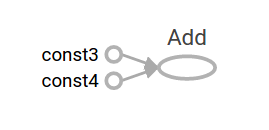
For more about TensorBoard's graph visualization tools see @{$graph_viz}.

### Session

To evaluate tensors, instantiate a `tf.Session` object, informally known as a
**session**. A session encapsulates the state of the TensorFlow runtime, and
runs TensorFlow operations. If a `tf.Graph` is like a `.py` file, a `tf.Session`
is like the `python` executable.

The following code creates a `tf.Session` object and then invokes its `run`
method to evaluate the `total` tensor we created above:

```python
sess = tf.Session()
print(sess.run(total))
```

When you request the output of a node with `Session.run` TensorFlow backtracks
through the graph and runs all the nodes that provide input to the requested
output node. So this prints the expected value of 7.0:

```
7.0
```

You can pass multiple tensors to `tf.Session.run`. The `run` method
transparently handles any combination of tuples or dictionaries, as in the
following example:

```python
print(sess.run({'ab':(a, b), 'total':total}))
```

which returns the results in a structure of the same layout:

``` None
{'total': 7.0, 'ab': (3.0, 4.0)}
```

During a call to `tf.Session.run` any `tf.Tensor` only has a single value.
For example, the following code calls `tf.random_uniform` to produce a
`tf.Tensor` that generates a random 3-element vector (with values in `[0,1)`):

```python
vec = tf.random_uniform(shape=(3,))
out1 = vec + 1
out2 = vec + 2
print(sess.run(vec))
print(sess.run(vec))
print(sess.run((out1, out2)))
```

The result shows a different random value on each call to `run`, but
a consistent value during a single `run` (`out1` and `out2` receive the same
random input):

```
[ 0.52917576  0.64076328  0.68353939]
[ 0.66192627  0.89126778  0.06254101]
(
  array([ 1.88408756,  1.87149239,  1.84057522], dtype=float32),
  array([ 2.88408756,  2.87149239,  2.84057522], dtype=float32)
)
```

Some TensorFlow functions return `tf.Operations` instead of `tf.Tensors`.
The result of calling `run` on an Operation is `None`. You run an operation
to cause a side-effect, not to retrieve a value. Examples of this include the
[initialization](#Initializing Layers), and [training](#Training) ops
demonstrated later.

### Feeding

As it stands, this graph is not especially interesting because it always
produces a constant result. A graph can be parameterized to accept external
inputs, known as **placeholders**. A **placeholder** is a promise to provide a
value later, like a function argument.

```python
x = tf.placeholder(tf.float32)
y = tf.placeholder(tf.float32)
z = x + y
```

The preceding three lines are a bit like a function in which we
define two input parameters (`x` and `y`) and then an operation on them. We can
evaluate this graph with multiple inputs by using the `feed_dict` argument of
the `tf.Session.run` method to feed concrete values to the placeholders:

```python
print(sess.run(z, feed_dict={x: 3, y: 4.5}))
print(sess.run(z, feed_dict={x: [1, 3], y: [2, 4]}))
```
This results in the following output:

```
7.5
[ 3.  7.]
```

Also note that the `feed_dict` argument can be used to overwrite any tensor in
the graph. The only difference between placeholders and other `tf.Tensors` is
that placeholders throw an error if no value is fed to them.

## Datasets

Placeholders work for simple experiments, but `tf.data` are the
preferred method of streaming data into a model.

To get a runnable `tf.Tensor` from a Dataset you must first convert it to a
`tf.data.Iterator`, and then call the Iterator's
`tf.data.Iterator.get_next` method.

The simplest way to create an Iterator is with the
`tf.data.Dataset.make_one_shot_iterator` method.
For example, in the following code the `next_item` tensor will return a row from
the `my_data` array on each `run` call:

``` python
my_data = [
    [0, 1,],
    [2, 3,],
    [4, 5,],
    [6, 7,],
]
slices = tf.data.Dataset.from_tensor_slices(my_data)
next_item = slices.make_one_shot_iterator().get_next()
```

Reaching the end of the data stream causes `Dataset` to throw an
`tf.errors.OutOfRangeError`. For example, the following code
reads the `next_item` until there is no more data to read:

``` python
while True:
  try:
    print(sess.run(next_item))
  except tf.errors.OutOfRangeError:
    break
```

If the `Dataset` depends on stateful operations you may need to
initialize the iterator before using it, as shown below:

``` python
r = tf.random_normal([10,3])
dataset = tf.data.Dataset.from_tensor_slices(r)
iterator = dataset.make_initializable_iterator()
next_row = iterator.get_next()

sess.run(iterator.initializer)
while True:
  try:
    print(sess.run(next_row))
  except tf.errors.OutOfRangeError:
    break
```

For more details on Datasets and Iterators see: @{$guide/datasets}.

## Layers

A trainable model must modify the values in the graph to get new outputs with
the same input.  `tf.layers` are the preferred way to add trainable
parameters to a graph.

Layers package together both the variables and the operations that act
on them. For example a
[densely-connected layer](https://developers.google.com/machine-learning/glossary/#fully_connected_layer)
performs a weighted sum across all inputs
for each output and applies an optional
[activation function](https://developers.google.com/machine-learning/glossary/#activation_function).
The connection weights and biases are managed by the layer object.

### Creating Layers

The following code creates a `tf.layers.Dense` layer that takes a
batch of input vectors, and produces a single output value for each. To apply a
layer to an input, call the layer as if it were a function. For example:

```python
x = tf.placeholder(tf.float32, shape=[None, 3])
linear_model = tf.layers.Dense(units=1)
y = linear_model(x)
```

The layer inspects its input to determine sizes for its internal variables. So
here we must set the shape of the `x` placeholder so that the layer can
build a weight matrix of the correct size.

Now that we have defined the calculation of the output, `y`, there is one more
detail we need to take care of before we run the calculation.

### Initializing Layers

The layer contains variables that must be **initialized** before they can be
used. While it is possible to initialize variables individually, you can easily
initialize all the variables in a TensorFlow graph as follows:

```python
init = tf.global_variables_initializer()
sess.run(init)
```

Important: Calling `tf.global_variables_initializer` only
creates and returns a handle to a TensorFlow operation. That op
will initialize all the global variables when we run it with `tf.Session.run`.

Also note that this `global_variables_initializer` only initializes variables
that existed in the graph when the  initializer was created. So the initializer
should be one of the last things added during graph construction.

### Executing Layers

Now that the layer is initialized, we can evaluate the `linear_model`'s output
tensor as we would any other tensor. For example, the following code:

```python
print(sess.run(y, {x: [[1, 2, 3],[4, 5, 6]]}))
```

will generate a two-element output vector such as the following:

```
[[-3.41378999]
 [-9.14999008]]
```

### Layer Function shortcuts

For each layer class (like `tf.layers.Dense`) TensorFlow also supplies a
shortcut function (like `tf.layers.dense`). The only difference is that the
shortcut function versions create and run the layer in a single call. For
example, the following code is equivalent to the earlier version:

```python
x = tf.placeholder(tf.float32, shape=[None, 3])
y = tf.layers.dense(x, units=1)

init = tf.global_variables_initializer()
sess.run(init)

print(sess.run(y, {x: [[1, 2, 3], [4, 5, 6]]}))
```

While convenient, this approach allows no access to the `tf.layers.Layer`
object. This makes introspection and debugging more difficult,
and layer reuse impossible.

## Feature columns

The easiest way to experiment with feature columns is using the
`tf.feature_column.input_layer` function. This function only accepts
@{$feature_columns$dense columns} as inputs, so to view the result
of a categorical column you must wrap it in an
`tf.feature_column.indicator_column`. For example:

``` python
features = {
    'sales' : [[5], [10], [8], [9]],
    'department': ['sports', 'sports', 'gardening', 'gardening']}

department_column = tf.feature_column.categorical_column_with_vocabulary_list(
        'department', ['sports', 'gardening'])
department_column = tf.feature_column.indicator_column(department_column)

columns = [
    tf.feature_column.numeric_column('sales'),
    department_column
]

inputs = tf.feature_column.input_layer(features, columns)
```

Running the `inputs` tensor will parse the `features` into a batch of vectors.

Feature columns can have internal state, like layers, so they often need to be
initialized. Categorical columns use `tf.contrib.lookup`
internally and these require a separate initialization op,
`tf.tables_initializer`.

``` python
var_init = tf.global_variables_initializer()
table_init = tf.tables_initializer()
sess = tf.Session()
sess.run((var_init, table_init))
```

Once the internal state has been initialized you can run `inputs` like any
other `tf.Tensor`:

```python
print(sess.run(inputs))
```

This shows how the feature columns have packed the input vectors, with the
one-hot "department" as the first two indices and "sales" as the third.

```None
[[  1.   0.   5.]
 [  1.   0.  10.]
 [  0.   1.   8.]
 [  0.   1.   9.]]
```

## Training

Now that you're familiar with the basics of core TensorFlow, let's train a
small regression model manually.

### Define the data

First let's define some inputs, `x`, and the expected output for each input,
`y_true`:

```python
x = tf.constant([[1], [2], [3], [4]], dtype=tf.float32)
y_true = tf.constant([[0], [-1], [-2], [-3]], dtype=tf.float32)
```

### Define the model

Next, build a simple linear model, with 1 output:

``` python
linear_model = tf.layers.Dense(units=1)

y_pred = linear_model(x)
```

You can evaluate the predictions as follows:

``` python
sess = tf.Session()
init = tf.global_variables_initializer()
sess.run(init)

print(sess.run(y_pred))
```

The model hasn't yet been trained, so the four "predicted" values aren't very
good. Here's what we got; your own output will almost certainly differ:

``` None
[[ 0.02631879]
 [ 0.05263758]
 [ 0.07895637]
 [ 0.10527515]]
```

### Loss

To optimize a model, you first need to define the loss. We'll use the mean
square error, a standard loss for regression problems.

While you could do this manually with lower level math operations,
the `tf.losses` module provides a set of common loss functions. You can use it
to calculate the mean square error as follows:

``` python
loss = tf.losses.mean_squared_error(labels=y_true, predictions=y_pred)

print(sess.run(loss))
```
This will produce a loss value, something like:

``` None
2.23962
```

### Training

TensorFlow provides
[**optimizers**](https://developers.google.com/machine-learning/glossary/#optimizer)
implementing standard optimization algorithms. These are implemented as
sub-classes of `tf.train.Optimizer`. They incrementally change each
variable in order to minimize the loss. The simplest optimization algorithm is
[**gradient descent**](https://developers.google.com/machine-learning/glossary/#gradient_descent),
implemented by `tf.train.GradientDescentOptimizer`. It modifies each
variable according to the magnitude of the derivative of loss with respect to
that variable. For example:

```python
optimizer = tf.train.GradientDescentOptimizer(0.01)
train = optimizer.minimize(loss)
```

This code builds all the graph components necessary for the optimization, and
returns a training operation. When run, the training op will update variables
in the graph. You might run it as follows:

```python
for i in range(100):
  _, loss_value = sess.run((train, loss))
  print(loss_value)
```

Since `train` is an op, not a tensor, it doesn't return a value when run.
To see the progression of the loss during training, we run the loss tensor at
the same time, producing output like the following:

``` None
1.35659
1.00412
0.759167
0.588829
0.470264
0.387626
0.329918
0.289511
0.261112
0.241046
...
```

### Complete program

```python
x = tf.constant([[1], [2], [3], [4]], dtype=tf.float32)
y_true = tf.constant([[0], [-1], [-2], [-3]], dtype=tf.float32)

linear_model = tf.layers.Dense(units=1)

y_pred = linear_model(x)
loss = tf.losses.mean_squared_error(labels=y_true, predictions=y_pred)

optimizer = tf.train.GradientDescentOptimizer(0.01)
train = optimizer.minimize(loss)

init = tf.global_variables_initializer()

sess = tf.Session()
sess.run(init)
for i in range(100):
  _, loss_value = sess.run((train, loss))
  print(loss_value)

print(sess.run(y_pred))
```

## Next steps

To learn more about building models with TensorFlow consider the following:

* @{$custom_estimators$Custom Estimators}, to learn how to build
  customized models with TensorFlow. Your knowledge of TensorFlow Core will
  help you understand and debug your own models.

If you want to learn more about the inner workings of TensorFlow consider the
following documents, which go into more depth on many of the topics discussed
here:

* @{$graphs}
* @{$tensors}
* @{$variables}