
diff options
Diffstat (limited to 'tensorflow/docs_src/guide/tensorboard_histograms.md')
| -rw-r--r-- | tensorflow/docs_src/guide/tensorboard_histograms.md | 245 |
1 files changed, 245 insertions, 0 deletions
diff --git a/tensorflow/docs_src/guide/tensorboard_histograms.md b/tensorflow/docs_src/guide/tensorboard_histograms.md new file mode 100644 index 0000000000..918deda190 --- /dev/null +++ b/tensorflow/docs_src/guide/tensorboard_histograms.md @@ -0,0 +1,245 @@ +# TensorBoard Histogram Dashboard + +The TensorBoard Histogram Dashboard displays how the distribution of some +`Tensor` in your TensorFlow graph has changed over time. It does this by showing +many histograms visualizations of your tensor at different points in time. + +## A Basic Example + +Let's start with a simple case: a normally-distributed variable, where the mean +shifts over time. +TensorFlow has an op +[`tf.random_normal`](https://www.tensorflow.org/api_docs/python/tf/random_normal) +which is perfect for this purpose. As is usually the case with TensorBoard, we +will ingest data using a summary op; in this case, +['tf.summary.histogram'](https://www.tensorflow.org/api_docs/python/tf/summary/histogram). +For a primer on how summaries work, please see the general +[TensorBoard tutorial](https://www.tensorflow.org/get_started/summaries_and_tensorboard). + +Here is a code snippet that will generate some histogram summaries containing +normally distributed data, where the mean of the distribution increases over +time. + +```python +import tensorflow as tf + +k = tf.placeholder(tf.float32) + +# Make a normal distribution, with a shifting mean +mean_moving_normal = tf.random_normal(shape=[1000], mean=(5*k), stddev=1) +# Record that distribution into a histogram summary +tf.summary.histogram("normal/moving_mean", mean_moving_normal) + +# Setup a session and summary writer +sess = tf.Session() +writer = tf.summary.FileWriter("/tmp/histogram_example") + +summaries = tf.summary.merge_all() + +# Setup a loop and write the summaries to disk +N = 400 +for step in range(N): + k_val = step/float(N) + summ = sess.run(summaries, feed_dict={k: k_val}) + writer.add_summary(summ, global_step=step) +``` + +Once that code runs, we can load the data into TensorBoard via the command line: + + +```sh +tensorboard --logdir=/tmp/histogram_example +``` + +Once TensorBoard is running, load it in Chrome or Firefox and navigate to the +Histogram Dashboard. Then we can see a histogram visualization for our normally +distributed data. + +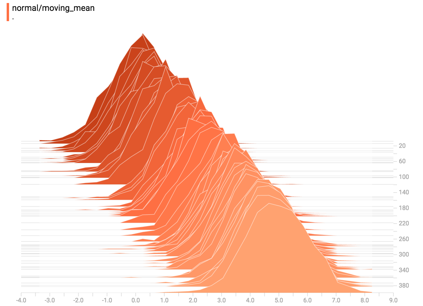 + +`tf.summary.histogram` takes an arbitrarily sized and shaped Tensor, and +compresses it into a histogram data structure consisting of many bins with +widths and counts. For example, let's say we want to organize the numbers +`[0.5, 1.1, 1.3, 2.2, 2.9, 2.99]` into bins. We could make three bins: +* a bin +containing everything from 0 to 1 (it would contain one element, 0.5), +* a bin +containing everything from 1-2 (it would contain two elements, 1.1 and 1.3), +* a bin containing everything from 2-3 (it would contain three elements: 2.2, +2.9 and 2.99). + +TensorFlow uses a similar approach to create bins, but unlike in our example, it +doesn't create integer bins. For large, sparse datasets, that might result in +many thousands of bins. +Instead, [the bins are exponentially distributed, with many bins close to 0 and +comparatively few bins for very large numbers.](https://github.com/tensorflow/tensorflow/blob/c8b59c046895fa5b6d79f73e0b5817330fcfbfc1/tensorflow/core/lib/histogram/histogram.cc#L28) +However, visualizing exponentially-distributed bins is tricky; if height is used +to encode count, then wider bins take more space, even if they have the same +number of elements. Conversely, encoding count in the area makes height +comparisons impossible. Instead, the histograms [resample the data](https://github.com/tensorflow/tensorflow/blob/17c47804b86e340203d451125a721310033710f1/tensorflow/tensorboard/components/tf_backend/backend.ts#L400) +into uniform bins. This can lead to unfortunate artifacts in some cases. + +Each slice in the histogram visualizer displays a single histogram. +The slices are organized by step; +older slices (e.g. step 0) are further "back" and darker, while newer slices +(e.g. step 400) are close to the foreground, and lighter in color. +The y-axis on the right shows the step number. + +You can mouse over the histogram to see tooltips with some more detailed +information. For example, in the following image we can see that the histogram +at timestep 176 has a bin centered at 2.25 with 177 elements in that bin. + +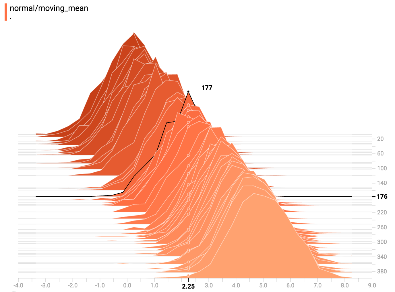 + +Also, you may note that the histogram slices are not always evenly spaced in +step count or time. This is because TensorBoard uses +[reservoir sampling](https://en.wikipedia.org/wiki/Reservoir_sampling) to keep a +subset of all the histograms, to save on memory. Reservoir sampling guarantees +that every sample has an equal likelihood of being included, but because it is +a randomized algorithm, the samples chosen don't occur at even steps. + +## Overlay Mode + +There is a control on the left of the dashboard that allows you to toggle the +histogram mode from "offset" to "overlay": + +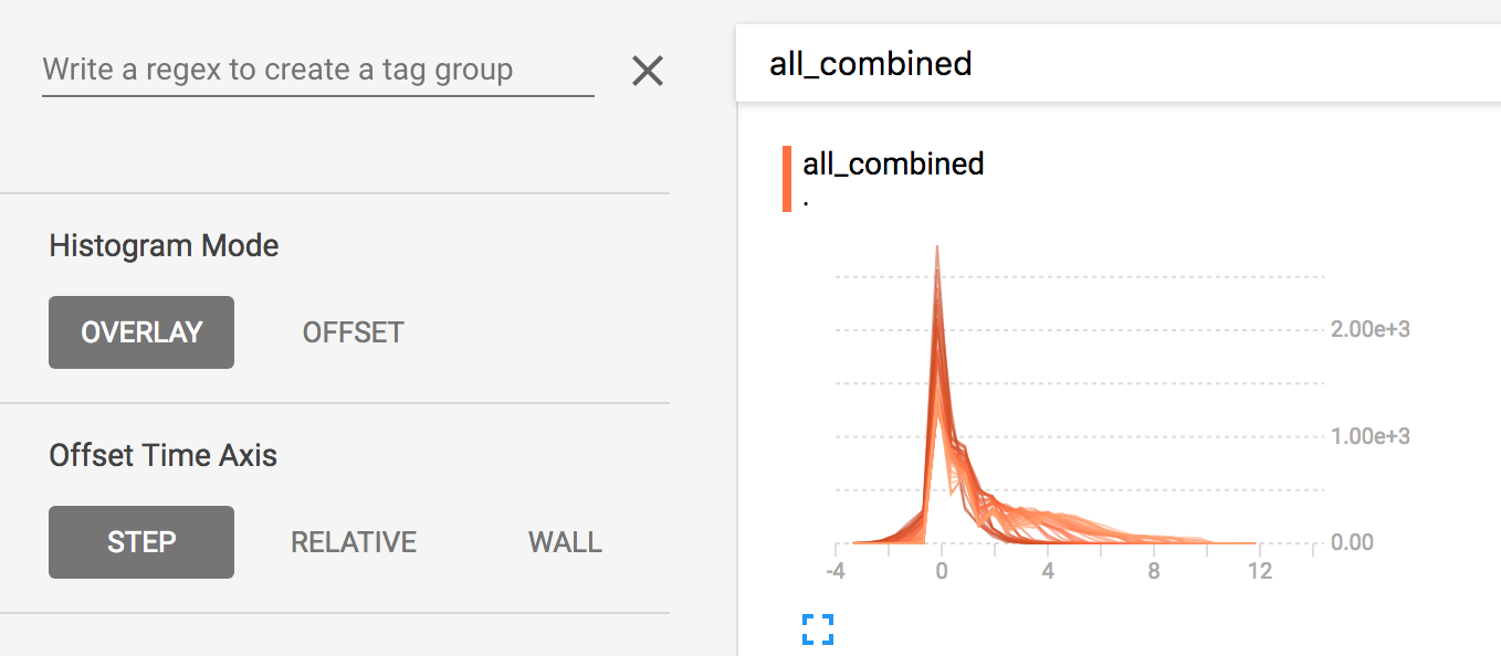 + +In "offset" mode, the visualization rotates 45 degrees, so that the individual +histogram slices are no longer spread out in time, but instead are all plotted +on the same y-axis. + +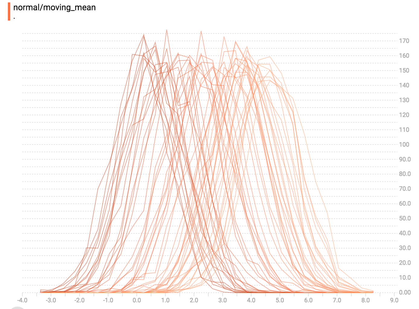 +Now, each slice is a separate line on the chart, and the y-axis shows the item +count within each bucket. Darker lines are older, earlier steps, and lighter +lines are more recent, later steps. Once again, you can mouse over the chart to +see some additional information. + +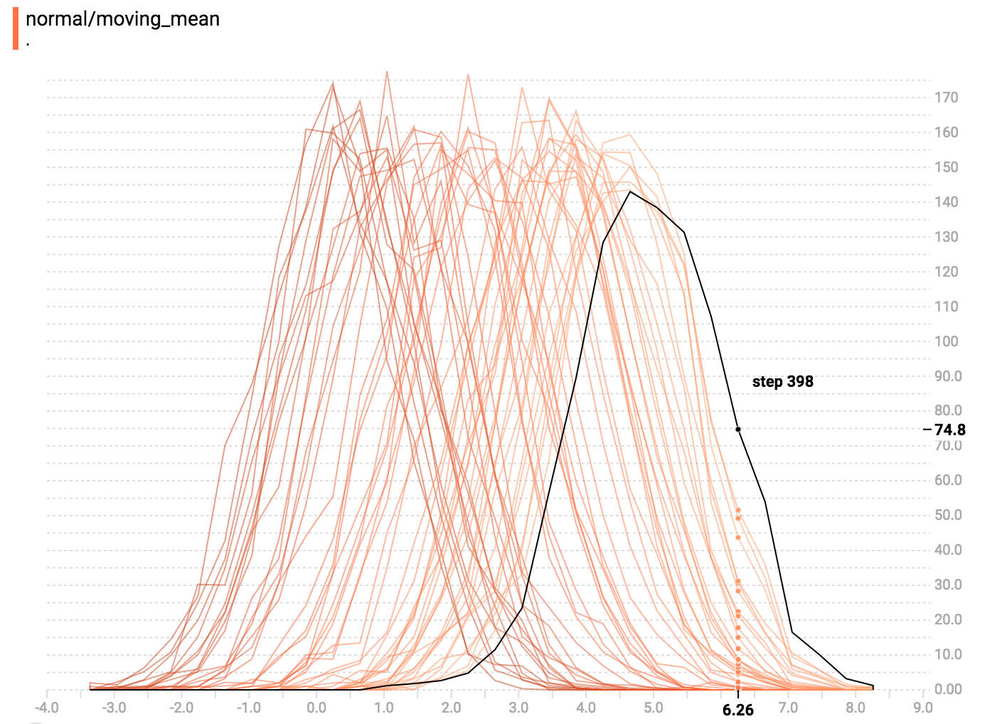 + +In general, the overlay visualization is useful if you want to directly compare +the counts of different histograms. + +## Multimodal Distributions + +The Histogram Dashboard is great for visualizing multimodal +distributions. Let's construct a simple bimodal distribution by concatenating +the outputs from two different normal distributions. The code will look like +this: + +```python +import tensorflow as tf + +k = tf.placeholder(tf.float32) + +# Make a normal distribution, with a shifting mean +mean_moving_normal = tf.random_normal(shape=[1000], mean=(5*k), stddev=1) +# Record that distribution into a histogram summary +tf.summary.histogram("normal/moving_mean", mean_moving_normal) + +# Make a normal distribution with shrinking variance +variance_shrinking_normal = tf.random_normal(shape=[1000], mean=0, stddev=1-(k)) +# Record that distribution too +tf.summary.histogram("normal/shrinking_variance", variance_shrinking_normal) + +# Let's combine both of those distributions into one dataset +normal_combined = tf.concat([mean_moving_normal, variance_shrinking_normal], 0) +# We add another histogram summary to record the combined distribution +tf.summary.histogram("normal/bimodal", normal_combined) + +summaries = tf.summary.merge_all() + +# Setup a session and summary writer +sess = tf.Session() +writer = tf.summary.FileWriter("/tmp/histogram_example") + +# Setup a loop and write the summaries to disk +N = 400 +for step in range(N): + k_val = step/float(N) + summ = sess.run(summaries, feed_dict={k: k_val}) + writer.add_summary(summ, global_step=step) +``` + +You already remember our "moving mean" normal distribution from the example +above. Now we also have a "shrinking variance" distribution. Side-by-side, they +look like this: +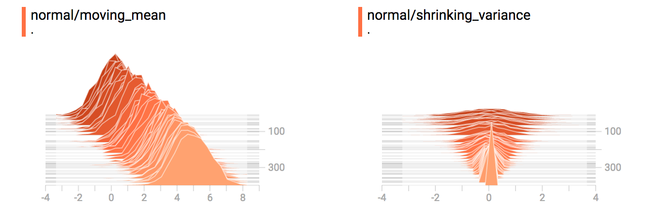 + +When we concatenate them, we get a chart that clearly reveals the divergent, +bimodal structure: +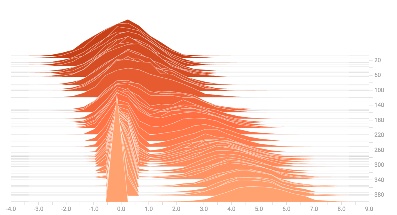 + +## Some more distributions + +Just for fun, let's generate and visualize a few more distributions, and then +combine them all into one chart. Here's the code we'll use: + +```python +import tensorflow as tf + +k = tf.placeholder(tf.float32) + +# Make a normal distribution, with a shifting mean +mean_moving_normal = tf.random_normal(shape=[1000], mean=(5*k), stddev=1) +# Record that distribution into a histogram summary +tf.summary.histogram("normal/moving_mean", mean_moving_normal) + +# Make a normal distribution with shrinking variance +variance_shrinking_normal = tf.random_normal(shape=[1000], mean=0, stddev=1-(k)) +# Record that distribution too +tf.summary.histogram("normal/shrinking_variance", variance_shrinking_normal) + +# Let's combine both of those distributions into one dataset +normal_combined = tf.concat([mean_moving_normal, variance_shrinking_normal], 0) +# We add another histogram summary to record the combined distribution +tf.summary.histogram("normal/bimodal", normal_combined) + +# Add a gamma distribution +gamma = tf.random_gamma(shape=[1000], alpha=k) +tf.summary.histogram("gamma", gamma) + +# And a poisson distribution +poisson = tf.random_poisson(shape=[1000], lam=k) +tf.summary.histogram("poisson", poisson) + +# And a uniform distribution +uniform = tf.random_uniform(shape=[1000], maxval=k*10) +tf.summary.histogram("uniform", uniform) + +# Finally, combine everything together! +all_distributions = [mean_moving_normal, variance_shrinking_normal, + gamma, poisson, uniform] +all_combined = tf.concat(all_distributions, 0) +tf.summary.histogram("all_combined", all_combined) + +summaries = tf.summary.merge_all() + +# Setup a session and summary writer +sess = tf.Session() +writer = tf.summary.FileWriter("/tmp/histogram_example") + +# Setup a loop and write the summaries to disk +N = 400 +for step in range(N): + k_val = step/float(N) + summ = sess.run(summaries, feed_dict={k: k_val}) + writer.add_summary(summ, global_step=step) +``` +### Gamma Distribution +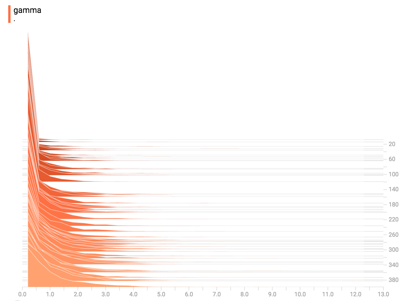 + +### Uniform Distribution +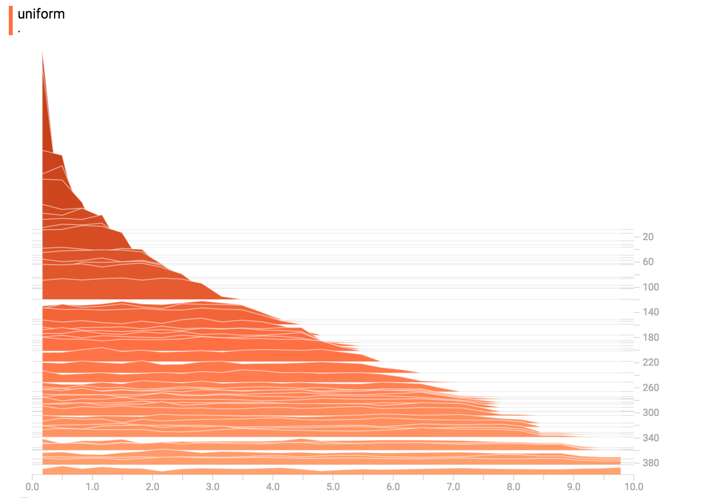 + +### Poisson Distribution +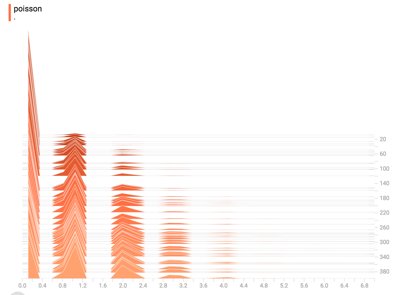 +The poisson distribution is defined over the integers. So, all of the values +being generated are perfect integers. The histogram compression moves the data +into floating-point bins, causing the visualization to show little +bumps over the integer values rather than perfect spikes. + +### All Together Now +Finally, we can concatenate all of the data into one funny-looking curve. +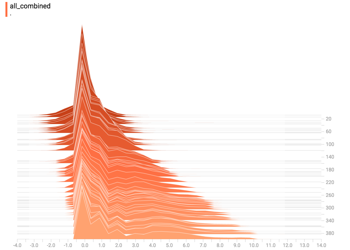 + |