
diff options
| author | 2018-01-11 16:38:14 -0800 | |
|---|---|---|
| committer | 2018-01-11 16:38:14 -0800 | |
| commit | aebb7cc8f5b065de06f9209a9b0b601b5b83cf70 (patch) | |
| tree | 559ab5b24663d2165d46df83a809a2d72e5f848b /tensorflow | |
| parent | 0a1cbfdc6d22b1d64b13a44abbc4a34f2fa02c84 (diff) | |
Apply 1.5-rc1 cherry-picks. (#16056)
* Delete empty api_guides.
PiperOrigin-RevId: 179215745
* Java: Instructions for using GPUs via Maven.
GPU support in Maven is being packaged with 1.5.0-rc0 onwards
(for Linux)
Fixes #12909
PiperOrigin-RevId: 180859336
* Fix build issues with cuda 9.1 through updating eigen. (#15796)
* Revert "Fix the headers error due to recent CUDA9.1 change (#15739)"
This reverts commit 3bc4900e7e60f43dc901523f1574f52440e7e701.
* Bump eigen dependency.
* Minor change to make tpu.rewrite compatible with Python 3.
AttrValue is a byte array, and handling this is different between Python 2 and 3.
PiperOrigin-RevId: 180306415
* TensorFlow for NVIDIA Tegra devices with CUDA support (#14167)
This commit enables CUDA support on compatible devices running Android such as the Nvidia TX1 and TX2 when using Makefile builds.
Note that JetPack for Android is required to build/run Android TF binaries with CUDA support. This should be released by Nvidia in the near future.
* Adding cuda_config.h to the pip package. (#15961)
* Adding cuda_config headers to our GPU build.
* Updating the local cuda path for cuda_headers.
* Removing the cuda_config blacklist.
* Buildifier fix.
* Ignoring .so files and manually adding the cuda_config.h file.
* Fixing the path for the src_dir.
* One last minor fix for path.
* Adding brackets.
* Minor fixes for "Linear" tutorial
PiperOrigin-RevId: 179061248
* Sync Premade and Custom estimator docs with example code.
PiperOrigin-RevId: 179404175
* rename files
PiperOrigin-RevId: 179683700
* Modernize old "get_started/get_started.md", as "programmers_guide/low_level_intro.md".
PiperOrigin-RevId: 179807033
* Add links to low level API intro
PiperOrigin-RevId: 179844300
* Make images larger
PiperOrigin-RevId: 181034398
* minor fixes to new "low_level_intro"
PiperOrigin-RevId: 181172455
* typo
PiperOrigin-RevId: 181185642
* Replace get_started
Also add sub-sections to leftnav files,
and sync leftnav and index files.
PiperOrigin-RevId: 181394206
* Added a "Getting Started with TensorFlow for ML Beginners" chapter to Get
Started section.
PiperOrigin-RevId: 181396430
* Add support for CUBLAS_TENSOR_OP_MATH in fp16 GEMM (#13451)
- Applies to matrix multiplications with fp16 input/output.
Computations will fall back to pseudo-fp16 if tensor op math is
disabled or not supported.
- Enabled by default. Tensor ops (both in cublas gemms and cudnn
convolutions) can be disabled globally by setting the
environment variable TF_DISABLE_TENSOR_OP_MATH=1. To disable
tensor ops specifically for gemms or convolutions use
TF_DISABLE_CUBLAS_TENSOR_OP_MATH=1 or
TF_DISABLE_CUDNN_TENSOR_OP_MATH=1, respectively.
- Added CUBLAS 9.0 algorithms to GetBlasGemmAlgorithms().
* Adding page to tensorflow.org with directions for building the TFLite demo on Android.
PiperOrigin-RevId: 179970218
Diffstat (limited to 'tensorflow')
72 files changed, 2182 insertions, 3825 deletions
diff --git a/tensorflow/contrib/copy_graph/__init__.py b/tensorflow/contrib/copy_graph/__init__.py index 30a0aac140..61ee39e4be 100644 --- a/tensorflow/contrib/copy_graph/__init__.py +++ b/tensorflow/contrib/copy_graph/__init__.py @@ -13,8 +13,6 @@ # limitations under the License. # ============================================================================== """Functions to copy elements between graphs. - -See the @{$python/contrib.copy_graph} guide. """ from __future__ import absolute_import diff --git a/tensorflow/contrib/makefile/Makefile b/tensorflow/contrib/makefile/Makefile index ee84b5b4c8..dd5770dc99 100644 --- a/tensorflow/contrib/makefile/Makefile +++ b/tensorflow/contrib/makefile/Makefile @@ -374,12 +374,72 @@ $(MARCH_OPTION) \ ifdef ENABLE_EXPERIMENTAL_HEXNN_OPS CXXFLAGS += -DENABLE_EXPERIMENTAL_HEXNN_OPS endif - - OBJDIR := $(OBJDIR)android_$(ANDROID_ARCH)/ - LIBDIR := $(LIBDIR)android_$(ANDROID_ARCH)/ - BINDIR := $(BINDIR)android_$(ANDROID_ARCH)/ - DEPDIR := $(DEPDIR)android_$(ANDROID_ARCH)/ + ifeq ($(BUILD_FOR_TEGRA),1) + NVCC := $(JETPACK)/cuda/bin/nvcc + NVCCFLAGS := -x=cu -D__CUDACC__ -DNVCC -DNVIDIA_TEGRA -ccbin $(NDK_ROOT)/toolchains/$(TOOLCHAIN)/prebuilt/$(ANDROID_HOST_OS_ARCH)/bin/$(BIN_PREFIX)-g++ --std c++11 --expt-relaxed-constexpr -m64 -gencode arch=compute_53,\"code=sm_53\" -gencode arch=compute_62,\"code=sm_62\" -DEIGEN_AVOID_STL_ARRAY -DTENSORFLOW_USE_EIGEN_THREADPOOL -DLANG_CXX11 -DEIGEN_HAS_C99_MATH -DGOOGLE_CUDA=1 -DTF_EXTRA_CUDA_CAPABILITIES=5.3 + CXXFLAGS4NVCC =\ +-DIS_SLIM_BUILD \ +-DNVIDIA_TEGRA \ +-fno-exceptions \ +-DNDEBUG $(OPTFLAGS) \ +-march=armv8-a \ +-fPIE \ +-D__ANDROID_TYPES_FULL__ \ +--sysroot $(NDK_ROOT)/platforms/android-21/arch-arm64 + + CXXFLAGS +=\ +-DGOOGLE_CUDA=1 \ +-D__ANDROID_TYPES_FULL__ \ +-DNVIDIA_TEGRA \ +-DEIGEN_AVOID_STL_ARRAY \ +-DEIGEN_HAS_C99_MATH \ +-DLANG_CXX11 -DTENSORFLOW_USE_EIGEN_THREADPOOL -DTF_EXTRA_CUDA_CAPABILITIES=5.3 + + INCLUDES += \ +-Itensorflow/core/kernels \ +-I$(MAKEFILE_DIR)/downloads/cub \ +-I$(MAKEFILE_DIR)/downloads/cub/cub_archive/cub/device \ +-Ithird_party/toolchains/gpus/cuda \ +-I$(JETPACK)/cuda/include \ +-I$(JETPACK) \ +-I$(JETPACK)/cuDNN/aarch64 \ +-I$(JETPACK)/cuda/extras/CUPTI/include + + + LIBS += \ +-ltfcuda \ +-lcudart_static \ +-lcudnn \ +-lcublas_static \ +-lcufftw_static \ +-lcusolver_static \ +-lcusparse_static \ +-lcufft \ +-lcuda \ +-lculibos \ +-lcurand_static + + OBJDIR := $(OBJDIR)Tegra/ + LIBDIR := $(LIBDIR)Tegra/ + BINDIR := $(BINDIR)Tegra/ + DEPDIR := $(DEPDIR)Tegra/ + + TEGRA_LIBS := \ +-L$(JETPACK)/cuda/targets/aarch64-linux-androideabi/lib \ +-L$(JETPACK)/cuda/targets/aarch64-linux-androideabi/lib/stubs \ +-L$(JETPACK)/cuda/targets/aarch64-linux-androideabi/lib64 \ +-L$(JETPACK)/cuda/targets/aarch64-linux-androideabi/lib64/stubs \ +-L$(JETPACK)/cuDNN/aarch64/cuda/lib64 \ +-L$(LIBDIR) + + CUDA_LIB_DEPS := $(LIBDIR)libtfcuda.a + else + OBJDIR := $(OBJDIR)android_$(ANDROID_ARCH)/ + LIBDIR := $(LIBDIR)android_$(ANDROID_ARCH)/ + BINDIR := $(BINDIR)android_$(ANDROID_ARCH)/ + DEPDIR := $(DEPDIR)android_$(ANDROID_ARCH)/ + endif # ifeq ($(BUILD_FOR_TEGRA),1) endif # ANDROID # LINT.ThenChange(//tensorflow/contrib/android/cmake/CMakeLists.txt) @@ -585,6 +645,65 @@ $(wildcard tensorflow/core/common_runtime/gpu_device_factory.*) \ $(wildcard tensorflow/core/grappler/inputs/trivial_test_graph_input_yielder.*) \ $(wildcard tensorflow/core/grappler/inputs/file_input_yielder.*) \ $(wildcard tensorflow/core/grappler/clusters/single_machine.*) + +ifeq ($(BUILD_FOR_TEGRA),1) +CORE_CC_ALL_SRCS := \ +$(wildcard tensorflow/core/*.cc) \ +$(wildcard tensorflow/core/common_runtime/*.cc) \ +$(wildcard tensorflow/core/common_runtime/gpu/*.cc) \ +$(wildcard tensorflow/core/framework/*.cc) \ +$(wildcard tensorflow/core/graph/*.cc) \ +$(wildcard tensorflow/core/platform/*.cc) \ +$(wildcard tensorflow/core/platform/*/*.cc) \ +$(wildcard tensorflow/core/platform/*/*/*.cc) \ +$(wildcard tensorflow/core/util/*.cc) \ +$(wildcard tensorflow/core/util/*/*.cc) \ +$(wildcard tensorflow/cc/training/*.cc) \ +$(wildcard tensorflow/stream_executor/*.cc) \ +$(wildcard tensorflow/stream_executor/*/*.cc) \ +$(wildcard tensorflow/core/grappler/optimizers/*.cc) \ +$(wildcard tensorflow/core/grappler/*.cc) \ +$(wildcard tensorflow/core/grappler/costs/*.cc) \ +$(wildcard tensorflow/core/grappler/clusters/*.cc) \ +$(wildcard tensorflow/core/grappler/utils/*.cc) \ +$(wildcard tensorflow/core/lib/core/*.cc) \ +$(wildcard tensorflow/core/lib/*/*.cc) \ +tensorflow/core/grappler/inputs/utils.cc \ +tensorflow/core/kernels/concat_lib_gpu.cc \ +tensorflow/core/kernels/cuda_solvers.cc \ +tensorflow/core/kernels/cudnn_pooling_gpu.cc \ +tensorflow/core/kernels/dense_update_functor.cc \ +tensorflow/core/kernels/fractional_avg_pool_op.cc \ +tensorflow/core/kernels/fractional_max_pool_op.cc \ +tensorflow/core/kernels/fractional_pool_common.cc \ +tensorflow/core/kernels/pooling_ops_3d.cc \ +tensorflow/core/kernels/sparse_fill_empty_rows_op.cc + +CORE_CC_EXCLUDE_SRCS := \ +$(wildcard tensorflow/core/*/*test.cc) \ +$(wildcard tensorflow/core/*/*testutil*) \ +$(wildcard tensorflow/core/*/*testlib*) \ +$(wildcard tensorflow/core/*/*/*test.cc) \ +$(wildcard tensorflow/core/*/*/*testutil*) \ +$(wildcard tensorflow/core/framework/op_gen_lib.cc) \ +$(wildcard tensorflow/core/lib/gif/*) \ +$(wildcard tensorflow/core/lib/jpeg/*) \ +$(wildcard tensorflow/core/lib/png/*) \ +$(wildcard tensorflow/core/lib/db/*) \ +$(wildcard tensorflow/core/platform/jpeg.*) \ +$(wildcard tensorflow/core/platform/png.*) \ +$(wildcard tensorflow/core/platform/cloud/*) \ +$(wildcard tensorflow/core/platform/s3/*) \ +$(wildcard tensorflow/core/platform/windows/*) \ +$(wildcard tensorflow/core/*/*/*testlib*) \ +$(wildcard tensorflow/cc/training/*test.cc) \ +tensorflow/core/lib/io/record_reader.cc \ +tensorflow/core/util/cuda_kernel_helper_test.cu.cc + +CUDA_CC_SRCS := $(wildcard tensorflow/core/kernels/*.cu.cc) +CUDA_CC_OBJS := $(addprefix $(OBJDIR), $(CUDA_CC_SRCS:.cc=.o)) +endif # TEGRA + # Filter out all the excluded files. TF_CC_SRCS := $(filter-out $(CORE_CC_EXCLUDE_SRCS), $(CORE_CC_ALL_SRCS)) # Add in any extra files that don't fit the patterns easily @@ -637,11 +756,23 @@ $(LIB_PATH): $(LIB_OBJS) @mkdir -p $(dir $@) $(AR) $(ARFLAGS) $(LIB_PATH) $(LIB_OBJS) -$(BENCHMARK_NAME): $(BENCHMARK_OBJS) $(LIB_PATH) +$(BENCHMARK_NAME): $(BENCHMARK_OBJS) $(LIB_PATH) $(CUDA_LIB_DEPS) @mkdir -p $(dir $@) $(CXX) $(CXXFLAGS) $(INCLUDES) \ -o $(BENCHMARK_NAME) $(BENCHMARK_OBJS) \ - $(LIBFLAGS) $(LIB_PATH) $(LDFLAGS) $(LIBS) + $(LIBFLAGS) $(TEGRA_LIBS) $(LIB_PATH) $(LDFLAGS) $(LIBS) + +# NVCC compilation rules for Tegra +ifeq ($(BUILD_FOR_TEGRA),1) +$(OBJDIR)%.cu.o: %.cu.cc + @mkdir -p $(dir $@) + @mkdir -p $(dir $(DEPDIR)$*) + $(NVCC) $(NVCCFLAGS) -Xcompiler "$(CXXFLAGS4NVCC) $(DEPFLAGS)" $(INCLUDES) -c $< -o $@ + +$(LIBDIR)libtfcuda.a: $(CUDA_CC_OBJS) + @mkdir -p $(dir $@) + $(AR) $(ARFLAGS) $@ $(CUDA_CC_OBJS) +endif # Matches on the normal hand-written TensorFlow C++ source files. $(OBJDIR)%.o: %.cc | $(PBT_GEN_FILES) @@ -730,6 +861,7 @@ clean_except_protobuf_libs: cleantarget: rm -rf $(OBJDIR) rm -rf $(BINDIR) + rm -rf $(LIBDIR) $(DEPDIR)/%.d: ; .PRECIOUS: $(DEPDIR)/%.d diff --git a/tensorflow/contrib/makefile/build_all_android.sh b/tensorflow/contrib/makefile/build_all_android.sh index 81cb17a311..980a44a595 100755 --- a/tensorflow/contrib/makefile/build_all_android.sh +++ b/tensorflow/contrib/makefile/build_all_android.sh @@ -26,7 +26,7 @@ usage() { echo "-x [hexagon library path] copy and hexagon libraries in the specified path" echo "-a [architecture] Architecture of target android [default=armeabi-v7a] \ (supported architecture list: \ -arm64-v8a armeabi armeabi-v7a mips mips64 x86 x86_64)" +arm64-v8a armeabi armeabi-v7a mips mips64 x86 x86_64 tegra)" exit 1 } @@ -50,6 +50,26 @@ while getopts "Es:t:Tx:a:" opt_name; do done shift $((OPTIND - 1)) +if [ "$ARCH" == "tegra" ]; then + if [[ -z "${JETPACK}" ]]; then + export JETPACK="$HOME/JetPack_Android_3.0" + fi + if [ ! -d ${JETPACK} ]; then + echo "Can't find Jetpack at ${JETPACK}" + echo "Set JETPACK=<path to Jetpack Android> to specify a non-default Jetpack path" + exit -1 + fi + if [ ! -d ${JETPACK}/cuda ]; then + ln -s $(ls -d ${JETPACK}/cuda-*/|sort -r|head -n1) ${JETPACK}/cuda + fi + if [ ! -d ${JETPACK}/cuda ]; then + ln -s $(ls -d ${JETPACK}/cuda-*/|sort -r|head -n1) ${JETPACK}/cuda + fi + + export BUILD_FOR_TEGRA=1 + ARCH="arm64-v8a" +fi + # Make sure we're in the correct directory, at the root of the source tree. SCRIPT_DIR="$(cd "$(dirname "${BASH_SOURCE[0]}")" >/dev/null && pwd)" cd "${SCRIPT_DIR}"/../../../ diff --git a/tensorflow/contrib/makefile/download_dependencies.sh b/tensorflow/contrib/makefile/download_dependencies.sh index b610441308..0a47f50c43 100755 --- a/tensorflow/contrib/makefile/download_dependencies.sh +++ b/tensorflow/contrib/makefile/download_dependencies.sh @@ -34,6 +34,7 @@ PROTOBUF_URL="$(grep -o 'https://mirror.bazel.build/github.com/google/protobuf/. RE2_URL="$(grep -o 'https://mirror.bazel.build/github.com/google/re2/.*tar\.gz' "${BZL_FILE_PATH}" | head -n1)" FFT2D_URL="$(grep -o 'http.*fft\.tgz' "${BZL_FILE_PATH}" | grep -v mirror.bazel | head -n1)" ABSL_URL="$(grep -o 'https://github.com/abseil/abseil-cpp/.*tar.gz' "${BZL_FILE_PATH}" | head -n1)" +CUB_URL="$(grep -o 'https.*cub/archive.*zip' "${BZL_FILE_PATH}" | grep -v bazel-mirror | head -n1)" # TODO(petewarden): Some new code in Eigen triggers a clang bug with iOS arm64, # so work around it by patching the source. @@ -82,6 +83,7 @@ download_and_extract "${PROTOBUF_URL}" "${DOWNLOADS_DIR}/protobuf" download_and_extract "${RE2_URL}" "${DOWNLOADS_DIR}/re2" download_and_extract "${FFT2D_URL}" "${DOWNLOADS_DIR}/fft2d" download_and_extract "${ABSL_URL}" "${DOWNLOADS_DIR}/absl" +download_and_extract "${CUB_URL}" "${DOWNLOADS_DIR}/cub/external/cub_archive" replace_by_sed 's#static uint32x4_t p4ui_CONJ_XOR = vld1q_u32( conj_XOR_DATA );#static uint32x4_t p4ui_CONJ_XOR; // = vld1q_u32( conj_XOR_DATA ); - Removed by script#' \ "${DOWNLOADS_DIR}/eigen/Eigen/src/Core/arch/NEON/Complex.h" diff --git a/tensorflow/contrib/makefile/sub_makefiles/android/Makefile.in b/tensorflow/contrib/makefile/sub_makefiles/android/Makefile.in index 26c1ad4947..d9277ed60c 100644 --- a/tensorflow/contrib/makefile/sub_makefiles/android/Makefile.in +++ b/tensorflow/contrib/makefile/sub_makefiles/android/Makefile.in @@ -48,10 +48,10 @@ INFERENCE_OBJS := $(addprefix $(OBJDIR), $(INFERENCE_SRCS:.cc=.o)) INFERENCE_SO_NAME := libtensorflow_inference.so INFERENCE_SO_PATH := $(LIBDIR)$(INFERENCE_SO_NAME) -$(INFERENCE_SO_PATH): $(LIB_OBJS) $(INFERENCE_OBJS) +$(INFERENCE_SO_PATH): $(LIB_OBJS) $(INFERENCE_OBJS) $(CUDA_LIB_DEPS) @mkdir -p $(dir $@) $(CXX) $(CXXFLAGS) $(INCLUDES) \ - -o $@ $(INFERENCE_OBJS) $(LIB_OBJS) \ + -o $@ $(INFERENCE_OBJS) $(LIB_OBJS) $(TEGRA_LIBS) \ $(LIBFLAGS) $(LDFLAGS) \ -shared -Wl,-soname,$(INFERENCE_SO_NAME) \ $(LIBS) diff --git a/tensorflow/contrib/tpu/python/tpu/tpu.py b/tensorflow/contrib/tpu/python/tpu/tpu.py index 7fb8a33698..7569c29f05 100644 --- a/tensorflow/contrib/tpu/python/tpu/tpu.py +++ b/tensorflow/contrib/tpu/python/tpu/tpu.py @@ -30,6 +30,7 @@ from tensorflow.python.ops import array_ops from tensorflow.python.ops import control_flow_ops from tensorflow.python.ops import variable_scope from tensorflow.python.platform import tf_logging as logging +from tensorflow.python.util import compat # Operations that indicate some error in the users graph, e.g. a placeholder @@ -52,6 +53,10 @@ _NOT_IMPLEMENTED_OPS = set([ "TensorSummaryV2", ]) +_MAX_WARNING_LINES = 5 + +_TPU_REPLICATE_ATTR = "_tpu_replicate" + def _tpu_system_device_name(job): """Returns the device name for the TPU_SYSTEM device of `job`.""" @@ -119,6 +124,17 @@ class TPUReplicateContext(control_flow_ops.ControlFlowContext): def __init__(self, name): control_flow_ops.ControlFlowContext.__init__(self) self._name = name + self._unsupported_ops = [] + + def report_unsupported_operations(self): + if self._unsupported_ops: + op_str = "\n".join([" %s (%s)" % (op.type, op.name) + for op in self._unsupported_ops[:_MAX_WARNING_LINES]]) + logging.warning("%d unsupported operations found: \n%s", + len(self._unsupported_ops), op_str) + if len(self._unsupported_ops) > _MAX_WARNING_LINES: + logging.warning("... and %d more" % + (len(self._unsupported_ops) - _MAX_WARNING_LINES)) def AddOp(self, op): self._AddOpInternal(op) @@ -130,17 +146,16 @@ class TPUReplicateContext(control_flow_ops.ControlFlowContext): (op.type, op.name)) if op.type in _NOT_IMPLEMENTED_OPS: - logging.warning( - "Operation %s (%s) is not currently supported", op.type, op.name) + self._unsupported_ops.append(op) if any(x.dtype._is_ref_dtype for x in op.inputs): raise NotImplementedError( "Non-resource Variables are not supported inside TPU computations " "(operator name: %s)" % op.name) # pylint: enable=protected-access - if "_tpu_replicate" in op.node_def.attr: + if _TPU_REPLICATE_ATTR in op.node_def.attr: raise ValueError("TPU computations cannot be nested") - op.node_def.attr["_tpu_replicate"].s = self._name + op.node_def.attr[_TPU_REPLICATE_ATTR].s = compat.as_bytes(self._name) op.graph.prevent_feeding(op) op.graph.prevent_fetching(op) @@ -344,6 +359,7 @@ def replicate(computation, new_output_tensors.append(array_ops.identity(t)) output_tensors = new_output_tensors finally: + context.report_unsupported_operations() context.Exit() # Fan-out: Builds a TPUReplicatedOutput node for each output. diff --git a/tensorflow/core/framework/register_types.h b/tensorflow/core/framework/register_types.h index 4bb37e4f6e..0f186a7a06 100644 --- a/tensorflow/core/framework/register_types.h +++ b/tensorflow/core/framework/register_types.h @@ -52,7 +52,7 @@ limitations under the License. #undef REGISTER_PARTITION */ -#if !defined(IS_MOBILE_PLATFORM) || defined(SUPPORT_SELECTIVE_REGISTRATION) +#if !defined(IS_MOBILE_PLATFORM) || defined(SUPPORT_SELECTIVE_REGISTRATION) || defined(NVIDIA_TEGRA) // All types are supported, so all macros are invoked. // diff --git a/tensorflow/docs_src/api_guides/python/client.md b/tensorflow/docs_src/api_guides/python/client.md index 97c1986360..eef23696db 100644 --- a/tensorflow/docs_src/api_guides/python/client.md +++ b/tensorflow/docs_src/api_guides/python/client.md @@ -3,8 +3,8 @@ This library contains classes for launching graphs and executing operations. -The @{$get_started/get_started} guide has -examples of how a graph is launched in a @{tf.Session}. +@{$programmers_guide/low_level_intro$This guide} has examples of how a graph +is launched in a @{tf.Session}. ## Session management diff --git a/tensorflow/docs_src/api_guides/python/contrib.bayesflow.entropy.md b/tensorflow/docs_src/api_guides/python/contrib.bayesflow.entropy.md deleted file mode 100644 index fc5d5d70d7..0000000000 --- a/tensorflow/docs_src/api_guides/python/contrib.bayesflow.entropy.md +++ /dev/null @@ -1 +0,0 @@ -# BayesFlow Entropy (contrib) diff --git a/tensorflow/docs_src/api_guides/python/contrib.bayesflow.stochastic_graph.md b/tensorflow/docs_src/api_guides/python/contrib.bayesflow.stochastic_graph.md deleted file mode 100644 index d855787ae6..0000000000 --- a/tensorflow/docs_src/api_guides/python/contrib.bayesflow.stochastic_graph.md +++ /dev/null @@ -1 +0,0 @@ -# BayesFlow Stochastic Graph (contrib) diff --git a/tensorflow/docs_src/api_guides/python/contrib.bayesflow.stochastic_tensor.md b/tensorflow/docs_src/api_guides/python/contrib.bayesflow.stochastic_tensor.md deleted file mode 100644 index 1cc1ac5d7e..0000000000 --- a/tensorflow/docs_src/api_guides/python/contrib.bayesflow.stochastic_tensor.md +++ /dev/null @@ -1,3 +0,0 @@ -# BayesFlow Stochastic Tensors (contrib) -[TOC] - diff --git a/tensorflow/docs_src/api_guides/python/contrib.bayesflow.variational_inference.md b/tensorflow/docs_src/api_guides/python/contrib.bayesflow.variational_inference.md deleted file mode 100644 index 8f08c09c8f..0000000000 --- a/tensorflow/docs_src/api_guides/python/contrib.bayesflow.variational_inference.md +++ /dev/null @@ -1,4 +0,0 @@ -# BayesFlow Variational Inference (contrib) -[TOC] - -Variational inference. diff --git a/tensorflow/docs_src/api_guides/python/contrib.copy_graph.md b/tensorflow/docs_src/api_guides/python/contrib.copy_graph.md deleted file mode 100644 index f61f4c764d..0000000000 --- a/tensorflow/docs_src/api_guides/python/contrib.copy_graph.md +++ /dev/null @@ -1,4 +0,0 @@ -# Copying Graph Elements (contrib) -[TOC] - -Functions for copying elements from one graph to another. diff --git a/tensorflow/docs_src/api_guides/python/contrib.opt.md b/tensorflow/docs_src/api_guides/python/contrib.opt.md deleted file mode 100644 index 944a80a5cc..0000000000 --- a/tensorflow/docs_src/api_guides/python/contrib.opt.md +++ /dev/null @@ -1,4 +0,0 @@ -# Optimization (contrib) -[TOC] - -opt: A module containing optimization routines. diff --git a/tensorflow/docs_src/api_guides/python/histogram_ops.md b/tensorflow/docs_src/api_guides/python/histogram_ops.md deleted file mode 100644 index dbd4555429..0000000000 --- a/tensorflow/docs_src/api_guides/python/histogram_ops.md +++ /dev/null @@ -1,6 +0,0 @@ -# Histograms -[TOC] - -## Histograms - -* @{tf.histogram_fixed_width} diff --git a/tensorflow/docs_src/api_guides/python/reading_data.md b/tensorflow/docs_src/api_guides/python/reading_data.md index f316cce953..b3ca958370 100644 --- a/tensorflow/docs_src/api_guides/python/reading_data.md +++ b/tensorflow/docs_src/api_guides/python/reading_data.md @@ -51,8 +51,7 @@ it is executed without a feed, so you won't forget to feed it. An example using `placeholder` and feeding to train on MNIST data can be found in -[`tensorflow/examples/tutorials/mnist/fully_connected_feed.py`](https://www.tensorflow.org/code/tensorflow/examples/tutorials/mnist/fully_connected_feed.py), -and is described in the @{$mechanics$MNIST tutorial}. +[`tensorflow/examples/tutorials/mnist/fully_connected_feed.py`](https://www.tensorflow.org/code/tensorflow/examples/tutorials/mnist/fully_connected_feed.py). ## `QueueRunner` diff --git a/tensorflow/docs_src/get_started/linear_regression.md b/tensorflow/docs_src/api_guides/python/regression_examples.md index 45cb9d829c..45cb9d829c 100644 --- a/tensorflow/docs_src/get_started/linear_regression.md +++ b/tensorflow/docs_src/api_guides/python/regression_examples.md diff --git a/tensorflow/docs_src/api_guides/python/script_ops.md b/tensorflow/docs_src/api_guides/python/script_ops.md deleted file mode 100644 index ab49a570c1..0000000000 --- a/tensorflow/docs_src/api_guides/python/script_ops.md +++ /dev/null @@ -1,13 +0,0 @@ -# Wraps python functions - -Note: Functions taking `Tensor` arguments can also take anything accepted by -@{tf.convert_to_tensor}. - -[TOC] - -## Script Language Operators - -TensorFlow provides allows you to wrap python/numpy functions as -TensorFlow operators. - -* @{tf.py_func} diff --git a/tensorflow/docs_src/deploy/distributed.md b/tensorflow/docs_src/deploy/distributed.md index f3e2fac49f..d7ed6b1deb 100644 --- a/tensorflow/docs_src/deploy/distributed.md +++ b/tensorflow/docs_src/deploy/distributed.md @@ -2,8 +2,8 @@ This document shows how to create a cluster of TensorFlow servers, and how to distribute a computation graph across that cluster. We assume that you are -familiar with the @{$get_started/get_started$basic concepts} of -writing TensorFlow programs. +familiar with the @{$programmers_guide/low_level_intro$basic concepts} of +writing low level TensorFlow programs. ## Hello distributed TensorFlow! diff --git a/tensorflow/docs_src/extend/architecture.md b/tensorflow/docs_src/extend/architecture.md index 21816502ac..c0fc714a44 100644 --- a/tensorflow/docs_src/extend/architecture.md +++ b/tensorflow/docs_src/extend/architecture.md @@ -7,7 +7,7 @@ learning models and system-level optimizations. This document describes the system architecture that makes possible this combination of scale and flexibility. It assumes that you have basic familiarity with TensorFlow programming concepts such as the computation graph, operations, -and sessions. See @{$get_started/get_started$Getting Started} +and sessions. See @{$programmers_guide/low_level_intro$this document} for an introduction to these topics. Some familiarity with @{$distributed$distributed TensorFlow} will also be helpful. diff --git a/tensorflow/docs_src/extend/estimators.md b/tensorflow/docs_src/extend/estimators.md deleted file mode 100644 index 96fc9fae47..0000000000 --- a/tensorflow/docs_src/extend/estimators.md +++ /dev/null @@ -1,698 +0,0 @@ -# Creating Estimators in tf.estimator - -The tf.estimator framework makes it easy to construct and train machine -learning models via its high-level Estimator API. `Estimator` -offers classes you can instantiate to quickly configure common model types such -as regressors and classifiers: - -* @{tf.estimator.LinearClassifier}: - Constructs a linear classification model. -* @{tf.estimator.LinearRegressor}: - Constructs a linear regression model. -* @{tf.estimator.DNNClassifier}: - Construct a neural network classification model. -* @{tf.estimator.DNNRegressor}: - Construct a neural network regression model. -* @{tf.estimator.DNNLinearCombinedClassifier}: - Construct a neural network and linear combined classification model. -* @{tf.estimator.DNNLinearCombinedRegressor}: - Construct a neural network and linear combined regression model. - -But what if none of `tf.estimator`'s predefined model types meets your needs? -Perhaps you need more granular control over model configuration, such as -the ability to customize the loss function used for optimization, or specify -different activation functions for each neural network layer. Or maybe you're -implementing a ranking or recommendation system, and neither a classifier nor a -regressor is appropriate for generating predictions. - -This tutorial covers how to create your own `Estimator` using the building -blocks provided in `tf.estimator`, which will predict the ages of -[abalones](https://en.wikipedia.org/wiki/Abalone) based on their physical -measurements. You'll learn how to do the following: - -* Instantiate an `Estimator` -* Construct a custom model function -* Configure a neural network using `tf.feature_column` and `tf.layers` -* Choose an appropriate loss function from `tf.losses` -* Define a training op for your model -* Generate and return predictions - -## Prerequisites - -This tutorial assumes you already know tf.estimator API basics, such as -feature columns, input functions, and `train()`/`evaluate()`/`predict()` -operations. If you've never used tf.estimator before, or need a refresher, -you should first review the following tutorials: - -* @{$get_started/estimator$tf.estimator Quickstart}: Quick introduction to - training a neural network using tf.estimator. -* @{$wide$TensorFlow Linear Model Tutorial}: Introduction to - feature columns, and an overview on building a linear classifier in - tf.estimator. -* @{$input_fn$Building Input Functions with tf.estimator}: Overview of how - to construct an input_fn to preprocess and feed data into your models. - -## An Abalone Age Predictor {#abalone-predictor} - -It's possible to estimate the age of an -[abalone](https://en.wikipedia.org/wiki/Abalone) (sea snail) by the number of -rings on its shell. However, because this task requires cutting, staining, and -viewing the shell under a microscope, it's desirable to find other measurements -that can predict age. - -The [Abalone Data Set](https://archive.ics.uci.edu/ml/datasets/Abalone) contains -the following -[feature data](https://archive.ics.uci.edu/ml/machine-learning-databases/abalone/abalone.names) -for abalone: - -| Feature | Description | -| -------------- | --------------------------------------------------------- | -| Length | Length of abalone (in longest direction; in mm) | -| Diameter | Diameter of abalone (measurement perpendicular to length; in mm)| -| Height | Height of abalone (with its meat inside shell; in mm) | -| Whole Weight | Weight of entire abalone (in grams) | -| Shucked Weight | Weight of abalone meat only (in grams) | -| Viscera Weight | Gut weight of abalone (in grams), after bleeding | -| Shell Weight | Weight of dried abalone shell (in grams) | - -The label to predict is number of rings, as a proxy for abalone age. - - -**[“Abalone shell”](https://www.flickr.com/photos/thenickster/16641048623/) (by [Nicki Dugan -Pogue](https://www.flickr.com/photos/thenickster/), CC BY-SA 2.0)** - -## Setup - -This tutorial uses three data sets. -[`abalone_train.csv`](http://download.tensorflow.org/data/abalone_train.csv) -contains labeled training data comprising 3,320 examples. -[`abalone_test.csv`](http://download.tensorflow.org/data/abalone_test.csv) -contains labeled test data for 850 examples. -[`abalone_predict`](http://download.tensorflow.org/data/abalone_predict.csv) -contains 7 examples on which to make predictions. - -The following sections walk through writing the `Estimator` code step by step; -the [full, final code is available -here](https://www.tensorflow.org/code/tensorflow/examples/tutorials/estimators/abalone.py). - -## Loading Abalone CSV Data into TensorFlow Datasets - -To feed the abalone dataset into the model, you'll need to download and load the -CSVs into TensorFlow `Dataset`s. First, add some standard Python and TensorFlow -imports, and set up FLAGS: - -```python -from __future__ import absolute_import -from __future__ import division -from __future__ import print_function - -import argparse -import sys -import tempfile - -# Import urllib -from six.moves import urllib - -import numpy as np -import tensorflow as tf - -FLAGS = None -``` - -Enable logging: - -```python -tf.logging.set_verbosity(tf.logging.INFO) -``` - -Then define a function to load the CSVs (either from files specified in -command-line options, or downloaded from -[tensorflow.org](https://www.tensorflow.org/)): - -```python -def maybe_download(train_data, test_data, predict_data): - """Maybe downloads training data and returns train and test file names.""" - if train_data: - train_file_name = train_data - else: - train_file = tempfile.NamedTemporaryFile(delete=False) - urllib.request.urlretrieve( - "http://download.tensorflow.org/data/abalone_train.csv", - train_file.name) - train_file_name = train_file.name - train_file.close() - print("Training data is downloaded to %s" % train_file_name) - - if test_data: - test_file_name = test_data - else: - test_file = tempfile.NamedTemporaryFile(delete=False) - urllib.request.urlretrieve( - "http://download.tensorflow.org/data/abalone_test.csv", test_file.name) - test_file_name = test_file.name - test_file.close() - print("Test data is downloaded to %s" % test_file_name) - - if predict_data: - predict_file_name = predict_data - else: - predict_file = tempfile.NamedTemporaryFile(delete=False) - urllib.request.urlretrieve( - "http://download.tensorflow.org/data/abalone_predict.csv", - predict_file.name) - predict_file_name = predict_file.name - predict_file.close() - print("Prediction data is downloaded to %s" % predict_file_name) - - return train_file_name, test_file_name, predict_file_name -``` - -Finally, create `main()` and load the abalone CSVs into `Datasets`, defining -flags to allow users to optionally specify CSV files for training, test, and -prediction datasets via the command line (by default, files will be downloaded -from [tensorflow.org](https://www.tensorflow.org/)): - -```python -def main(unused_argv): - # Load datasets - abalone_train, abalone_test, abalone_predict = maybe_download( - FLAGS.train_data, FLAGS.test_data, FLAGS.predict_data) - - # Training examples - training_set = tf.contrib.learn.datasets.base.load_csv_without_header( - filename=abalone_train, target_dtype=np.int, features_dtype=np.float64) - - # Test examples - test_set = tf.contrib.learn.datasets.base.load_csv_without_header( - filename=abalone_test, target_dtype=np.int, features_dtype=np.float64) - - # Set of 7 examples for which to predict abalone ages - prediction_set = tf.contrib.learn.datasets.base.load_csv_without_header( - filename=abalone_predict, target_dtype=np.int, features_dtype=np.float64) - -if __name__ == "__main__": - parser = argparse.ArgumentParser() - parser.register("type", "bool", lambda v: v.lower() == "true") - parser.add_argument( - "--train_data", type=str, default="", help="Path to the training data.") - parser.add_argument( - "--test_data", type=str, default="", help="Path to the test data.") - parser.add_argument( - "--predict_data", - type=str, - default="", - help="Path to the prediction data.") - FLAGS, unparsed = parser.parse_known_args() - tf.app.run(main=main, argv=[sys.argv[0]] + unparsed) -``` - -## Instantiating an Estimator - -When defining a model using one of tf.estimator's provided classes, such as -`DNNClassifier`, you supply all the configuration parameters right in the -constructor, e.g.: - -```python -my_nn = tf.estimator.DNNClassifier(feature_columns=[age, height, weight], - hidden_units=[10, 10, 10], - activation_fn=tf.nn.relu, - dropout=0.2, - n_classes=3, - optimizer="Adam") -``` - -You don't need to write any further code to instruct TensorFlow how to train the -model, calculate loss, or return predictions; that logic is already baked into -the `DNNClassifier`. - -By contrast, when you're creating your own estimator from scratch, the -constructor accepts just two high-level parameters for model configuration, -`model_fn` and `params`: - -```python -nn = tf.estimator.Estimator(model_fn=model_fn, params=model_params) -``` - -* `model_fn`: A function object that contains all the aforementioned logic to - support training, evaluation, and prediction. You are responsible for - implementing that functionality. The next section, [Constructing the - `model_fn`](#constructing-modelfn) covers creating a model function in - detail. - -* `params`: An optional dict of hyperparameters (e.g., learning rate, dropout) - that will be passed into the `model_fn`. - -Note: Just like `tf.estimator`'s predefined regressors and classifiers, the -`Estimator` initializer also accepts the general configuration arguments -`model_dir` and `config`. - -For the abalone age predictor, the model will accept one hyperparameter: -learning rate. Define `LEARNING_RATE` as a constant at the beginning of your -code (highlighted in bold below), right after the logging configuration: - -<pre class="prettyprint"><code class="lang-python">tf.logging.set_verbosity(tf.logging.INFO) - -<strong># Learning rate for the model -LEARNING_RATE = 0.001</strong></code></pre> - -Note: Here, `LEARNING_RATE` is set to `0.001`, but you can tune this value as -needed to achieve the best results during model training. - -Then, add the following code to `main()`, which creates the dict `model_params` -containing the learning rate and instantiates the `Estimator`: - -```python -# Set model params -model_params = {"learning_rate": LEARNING_RATE} - -# Instantiate Estimator -nn = tf.estimator.Estimator(model_fn=model_fn, params=model_params) -``` - -## Constructing the `model_fn` {#constructing-modelfn} - -The basic skeleton for an `Estimator` API model function looks like this: - -```python -def model_fn(features, labels, mode, params): - # Logic to do the following: - # 1. Configure the model via TensorFlow operations - # 2. Define the loss function for training/evaluation - # 3. Define the training operation/optimizer - # 4. Generate predictions - # 5. Return predictions/loss/train_op/eval_metric_ops in EstimatorSpec object - return EstimatorSpec(mode, predictions, loss, train_op, eval_metric_ops) -``` - -The `model_fn` must accept three arguments: - -* `features`: A dict containing the features passed to the model via - `input_fn`. -* `labels`: A `Tensor` containing the labels passed to the model via - `input_fn`. Will be empty for `predict()` calls, as these are the values the - model will infer. -* `mode`: One of the following @{tf.estimator.ModeKeys} string values - indicating the context in which the model_fn was invoked: - * `tf.estimator.ModeKeys.TRAIN` The `model_fn` was invoked in training - mode, namely via a `train()` call. - * `tf.estimator.ModeKeys.EVAL`. The `model_fn` was invoked in - evaluation mode, namely via an `evaluate()` call. - * `tf.estimator.ModeKeys.PREDICT`. The `model_fn` was invoked in - predict mode, namely via a `predict()` call. - -`model_fn` may also accept a `params` argument containing a dict of -hyperparameters used for training (as shown in the skeleton above). - -The body of the function performs the following tasks (described in detail in the -sections that follow): - -* Configuring the model—here, for the abalone predictor, this will be a neural - network. -* Defining the loss function used to calculate how closely the model's - predictions match the target values. -* Defining the training operation that specifies the `optimizer` algorithm to - minimize the loss values calculated by the loss function. - -The `model_fn` must return a @{tf.estimator.EstimatorSpec} -object, which contains the following values: - -* `mode` (required). The mode in which the model was run. Typically, you will - return the `mode` argument of the `model_fn` here. - -* `predictions` (required in `PREDICT` mode). A dict that maps key names of - your choice to `Tensor`s containing the predictions from the model, e.g.: - - ```python - predictions = {"results": tensor_of_predictions} - ``` - - In `PREDICT` mode, the dict that you return in `EstimatorSpec` will then be - returned by `predict()`, so you can construct it in the format in which - you'd like to consume it. - - -* `loss` (required in `EVAL` and `TRAIN` mode). A `Tensor` containing a scalar - loss value: the output of the model's loss function (discussed in more depth - later in [Defining loss for the model](#defining-loss)) calculated over all - the input examples. This is used in `TRAIN` mode for error handling and - logging, and is automatically included as a metric in `EVAL` mode. - -* `train_op` (required only in `TRAIN` mode). An Op that runs one step of - training. - -* `eval_metric_ops` (optional). A dict of name/value pairs specifying the - metrics that will be calculated when the model runs in `EVAL` mode. The name - is a label of your choice for the metric, and the value is the result of - your metric calculation. The @{tf.metrics} - module provides predefined functions for a variety of common metrics. The - following `eval_metric_ops` contains an `"accuracy"` metric calculated using - `tf.metrics.accuracy`: - - ```python - eval_metric_ops = { - "accuracy": tf.metrics.accuracy(labels, predictions) - } - ``` - - If you do not specify `eval_metric_ops`, only `loss` will be calculated - during evaluation. - -### Configuring a neural network with `tf.feature_column` and `tf.layers` - -Constructing a [neural -network](https://en.wikipedia.org/wiki/Artificial_neural_network) entails -creating and connecting the input layer, the hidden layers, and the output -layer. - -The input layer is a series of nodes (one for each feature in the model) that -will accept the feature data that is passed to the `model_fn` in the `features` -argument. If `features` contains an n-dimensional `Tensor` with all your feature -data, then it can serve as the input layer. -If `features` contains a dict of @{$linear#feature-columns-and-transformations$feature columns} passed to -the model via an input function, you can convert it to an input-layer `Tensor` -with the @{tf.feature_column.input_layer} function. - -```python -input_layer = tf.feature_column.input_layer( - features=features, feature_columns=[age, height, weight]) -``` - -As shown above, `input_layer()` takes two required arguments: - -* `features`. A mapping from string keys to the `Tensors` containing the - corresponding feature data. This is exactly what is passed to the `model_fn` - in the `features` argument. -* `feature_columns`. A list of all the `FeatureColumns` in the model—`age`, - `height`, and `weight` in the above example. - -The input layer of the neural network then must be connected to one or more -hidden layers via an [activation -function](https://en.wikipedia.org/wiki/Activation_function) that performs a -nonlinear transformation on the data from the previous layer. The last hidden -layer is then connected to the output layer, the final layer in the model. -`tf.layers` provides the `tf.layers.dense` function for constructing fully -connected layers. The activation is controlled by the `activation` argument. -Some options to pass to the `activation` argument are: - -* `tf.nn.relu`. The following code creates a layer of `units` nodes fully - connected to the previous layer `input_layer` with a - [ReLU activation function](https://en.wikipedia.org/wiki/Rectifier_\(neural_networks\)) - (@{tf.nn.relu}): - - ```python - hidden_layer = tf.layers.dense( - inputs=input_layer, units=10, activation=tf.nn.relu) - ``` - -* `tf.nn.relu6`. The following code creates a layer of `units` nodes fully - connected to the previous layer `hidden_layer` with a ReLU 6 activation - function (@{tf.nn.relu6}): - - ```python - second_hidden_layer = tf.layers.dense( - inputs=hidden_layer, units=20, activation=tf.nn.relu) - ``` - -* `None`. The following code creates a layer of `units` nodes fully connected - to the previous layer `second_hidden_layer` with *no* activation function, - just a linear transformation: - - ```python - output_layer = tf.layers.dense( - inputs=second_hidden_layer, units=3, activation=None) - ``` - -Other activation functions are possible, e.g.: - -```python -output_layer = tf.layers.dense(inputs=second_hidden_layer, - units=10, - activation_fn=tf.sigmoid) -``` - -The above code creates the neural network layer `output_layer`, which is fully -connected to `second_hidden_layer` with a sigmoid activation function -(@{tf.sigmoid}). For a list of predefined -activation functions available in TensorFlow, see the @{$python/nn#activation_functions$API docs}. - -Putting it all together, the following code constructs a full neural network for -the abalone predictor, and captures its predictions: - -```python -def model_fn(features, labels, mode, params): - """Model function for Estimator.""" - - # Connect the first hidden layer to input layer - # (features["x"]) with relu activation - first_hidden_layer = tf.layers.dense(features["x"], 10, activation=tf.nn.relu) - - # Connect the second hidden layer to first hidden layer with relu - second_hidden_layer = tf.layers.dense( - first_hidden_layer, 10, activation=tf.nn.relu) - - # Connect the output layer to second hidden layer (no activation fn) - output_layer = tf.layers.dense(second_hidden_layer, 1) - - # Reshape output layer to 1-dim Tensor to return predictions - predictions = tf.reshape(output_layer, [-1]) - predictions_dict = {"ages": predictions} - ... -``` - -Here, because you'll be passing the abalone `Datasets` using `numpy_input_fn` -as shown below, `features` is a dict `{"x": data_tensor}`, so -`features["x"]` is the input layer. The network contains two hidden -layers, each with 10 nodes and a ReLU activation function. The output layer -contains no activation function, and is -@{tf.reshape} to a one-dimensional -tensor to capture the model's predictions, which are stored in -`predictions_dict`. - -### Defining loss for the model {#defining-loss} - -The `EstimatorSpec` returned by the `model_fn` must contain `loss`: a `Tensor` -representing the loss value, which quantifies how well the model's predictions -reflect the label values during training and evaluation runs. The @{tf.losses} -module provides convenience functions for calculating loss using a variety of -metrics, including: - -* `absolute_difference(labels, predictions)`. Calculates loss using the - [absolute-difference - formula](https://en.wikipedia.org/wiki/Deviation_\(statistics\)#Unsigned_or_absolute_deviation) - (also known as L<sub>1</sub> loss). - -* `log_loss(labels, predictions)`. Calculates loss using the [logistic loss - forumula](https://en.wikipedia.org/wiki/Loss_functions_for_classification#Logistic_loss) - (typically used in logistic regression). - -* `mean_squared_error(labels, predictions)`. Calculates loss using the [mean - squared error](https://en.wikipedia.org/wiki/Mean_squared_error) (MSE; also - known as L<sub>2</sub> loss). - -The following example adds a definition for `loss` to the abalone `model_fn` -using `mean_squared_error()` (in bold): - -<pre class="prettyprint"><code class="lang-python">def model_fn(features, labels, mode, params): - """Model function for Estimator.""" - - # Connect the first hidden layer to input layer - # (features["x"]) with relu activation - first_hidden_layer = tf.layers.dense(features["x"], 10, activation=tf.nn.relu) - - # Connect the second hidden layer to first hidden layer with relu - second_hidden_layer = tf.layers.dense( - first_hidden_layer, 10, activation=tf.nn.relu) - - # Connect the output layer to second hidden layer (no activation fn) - output_layer = tf.layers.dense(second_hidden_layer, 1) - - # Reshape output layer to 1-dim Tensor to return predictions - predictions = tf.reshape(output_layer, [-1]) - predictions_dict = {"ages": predictions} - - - <strong># Calculate loss using mean squared error - loss = tf.losses.mean_squared_error(labels, predictions)</strong> - ...</code></pre> - -See the @{tf.losses$API guide} for a -full list of loss functions and more details on supported arguments and usage. - -Supplementary metrics for evaluation can be added to an `eval_metric_ops` dict. -The following code defines an `rmse` metric, which calculates the root mean -squared error for the model predictions. Note that the `labels` tensor is cast -to a `float64` type to match the data type of the `predictions` tensor, which -will contain real values: - -```python -eval_metric_ops = { - "rmse": tf.metrics.root_mean_squared_error( - tf.cast(labels, tf.float64), predictions) -} -``` - -### Defining the training op for the model - -The training op defines the optimization algorithm TensorFlow will use when -fitting the model to the training data. Typically when training, the goal is to -minimize loss. A simple way to create the training op is to instantiate a -`tf.train.Optimizer` subclass and call the `minimize` method. - -The following code defines a training op for the abalone `model_fn` using the -loss value calculated in [Defining Loss for the Model](#defining-loss), the -learning rate passed to the function in `params`, and the gradient descent -optimizer. For `global_step`, the convenience function -@{tf.train.get_global_step} takes care of generating an integer variable: - -```python -optimizer = tf.train.GradientDescentOptimizer( - learning_rate=params["learning_rate"]) -train_op = optimizer.minimize( - loss=loss, global_step=tf.train.get_global_step()) -``` - -For a full list of optimizers, and other details, see the -@{$python/train#optimizers$API guide}. - -### The complete abalone `model_fn` - -Here's the final, complete `model_fn` for the abalone age predictor. The -following code configures the neural network; defines loss and the training op; -and returns a `EstimatorSpec` object containing `mode`, `predictions_dict`, `loss`, -and `train_op`: - -```python -def model_fn(features, labels, mode, params): - """Model function for Estimator.""" - - # Connect the first hidden layer to input layer - # (features["x"]) with relu activation - first_hidden_layer = tf.layers.dense(features["x"], 10, activation=tf.nn.relu) - - # Connect the second hidden layer to first hidden layer with relu - second_hidden_layer = tf.layers.dense( - first_hidden_layer, 10, activation=tf.nn.relu) - - # Connect the output layer to second hidden layer (no activation fn) - output_layer = tf.layers.dense(second_hidden_layer, 1) - - # Reshape output layer to 1-dim Tensor to return predictions - predictions = tf.reshape(output_layer, [-1]) - - # Provide an estimator spec for `ModeKeys.PREDICT`. - if mode == tf.estimator.ModeKeys.PREDICT: - return tf.estimator.EstimatorSpec( - mode=mode, - predictions={"ages": predictions}) - - # Calculate loss using mean squared error - loss = tf.losses.mean_squared_error(labels, predictions) - - # Calculate root mean squared error as additional eval metric - eval_metric_ops = { - "rmse": tf.metrics.root_mean_squared_error( - tf.cast(labels, tf.float64), predictions) - } - - optimizer = tf.train.GradientDescentOptimizer( - learning_rate=params["learning_rate"]) - train_op = optimizer.minimize( - loss=loss, global_step=tf.train.get_global_step()) - - # Provide an estimator spec for `ModeKeys.EVAL` and `ModeKeys.TRAIN` modes. - return tf.estimator.EstimatorSpec( - mode=mode, - loss=loss, - train_op=train_op, - eval_metric_ops=eval_metric_ops) -``` - -## Running the Abalone Model - -You've instantiated an `Estimator` for the abalone predictor and defined its -behavior in `model_fn`; all that's left to do is train, evaluate, and make -predictions. - -Add the following code to the end of `main()` to fit the neural network to the -training data and evaluate accuracy: - -```python -train_input_fn = tf.estimator.inputs.numpy_input_fn( - x={"x": np.array(training_set.data)}, - y=np.array(training_set.target), - num_epochs=None, - shuffle=True) - -# Train -nn.train(input_fn=train_input_fn, steps=5000) - -# Score accuracy -test_input_fn = tf.estimator.inputs.numpy_input_fn( - x={"x": np.array(test_set.data)}, - y=np.array(test_set.target), - num_epochs=1, - shuffle=False) - -ev = nn.evaluate(input_fn=test_input_fn) -print("Loss: %s" % ev["loss"]) -print("Root Mean Squared Error: %s" % ev["rmse"]) -``` - -Note: The above code uses input functions to feed feature (`x`) and label (`y`) -`Tensor`s into the model for both training (`train_input_fn`) and evaluation -(`test_input_fn`). To learn more about input functions, see the tutorial -@{$input_fn$Building Input Functions with tf.estimator}. - -Then run the code. You should see output like the following: - -```none -... -INFO:tensorflow:loss = 4.86658, step = 4701 -INFO:tensorflow:loss = 4.86191, step = 4801 -INFO:tensorflow:loss = 4.85788, step = 4901 -... -INFO:tensorflow:Saving evaluation summary for 5000 step: loss = 5.581 -Loss: 5.581 -``` - -The loss score reported is the mean squared error returned from the `model_fn` -when run on the `ABALONE_TEST` data set. - -To predict ages for the `ABALONE_PREDICT` data set, add the following to -`main()`: - -```python -# Print out predictions -predict_input_fn = tf.estimator.inputs.numpy_input_fn( - x={"x": prediction_set.data}, - num_epochs=1, - shuffle=False) -predictions = nn.predict(input_fn=predict_input_fn) -for i, p in enumerate(predictions): - print("Prediction %s: %s" % (i + 1, p["ages"])) -``` - -Here, the `predict()` function returns results in `predictions` as an iterable. -The `for` loop enumerates and prints out the results. Rerun the code, and you -should see output similar to the following: - -```python -... -Prediction 1: 4.92229 -Prediction 2: 10.3225 -Prediction 3: 7.384 -Prediction 4: 10.6264 -Prediction 5: 11.0862 -Prediction 6: 9.39239 -Prediction 7: 11.1289 -``` - -## Additional Resources - -Congrats! You've successfully built a tf.estimator `Estimator` from scratch. -For additional reference materials on building `Estimator`s, see the following -sections of the API guides: - -* @{$python/contrib.layers$Layers} -* @{tf.losses$Losses} -* @{$python/contrib.layers#optimization$Optimization} diff --git a/tensorflow/docs_src/extend/index.md b/tensorflow/docs_src/extend/index.md index 00b168c6be..bdff60b39e 100644 --- a/tensorflow/docs_src/extend/index.md +++ b/tensorflow/docs_src/extend/index.md @@ -14,9 +14,6 @@ TensorFlow: add support for your own shared or distributed filesystem. * @{$new_data_formats$Custom Data Readers}, which details how to add support for your own file and record formats. - * @{$extend/estimators$Creating Estimators in tf.contrib.learn}, which explains how - to write your own custom Estimator. For example, you could build your - own Estimator to implement some variation on standard linear regression. Python is currently the only language supported by TensorFlow's API stability promises. However, TensorFlow also provides functionality in C++, Java, and Go, diff --git a/tensorflow/docs_src/extend/leftnav_files b/tensorflow/docs_src/extend/leftnav_files index 8dbb54f6f6..12315b711b 100644 --- a/tensorflow/docs_src/extend/leftnav_files +++ b/tensorflow/docs_src/extend/leftnav_files @@ -3,6 +3,5 @@ architecture.md adding_an_op.md add_filesys.md new_data_formats.md -estimators.md language_bindings.md tool_developers/index.md diff --git a/tensorflow/docs_src/get_started/saving_models.md b/tensorflow/docs_src/get_started/checkpoints.md index 056263c157..680e1c0d3f 100644 --- a/tensorflow/docs_src/get_started/saving_models.md +++ b/tensorflow/docs_src/get_started/checkpoints.md @@ -15,9 +15,8 @@ This document focuses on checkpoints. For details on SavedModel, see the ## Sample code -This document relies on the same Iris classification example detailed in -<!-- TODO (barryr): fill in link when module settles down. --> -@{$premade_estimators$Getting Started with TensorFlow}. +This document relies on the same +[https://github.com/tensorflow/models/blob/master/samples/core/get_started/premade_estimator.py](Iris classification example) detailed in @{$premade_estimators$Getting Started with TensorFlow}. To download and access the example, invoke the following two commands: ```shell @@ -228,10 +227,12 @@ This separation will keep your checkpoints recoverable. ## Summary -Checkpoints provide an easy automatic mechanism for storing and restoring -models created by Estimators. See the @{$saved_model$Saving and Restoring} +Checkpoints provide an easy automatic mechanism for saving and restoring +models created by Estimators. + +See the @{$saved_model$Saving and Restoring} chapter of the *TensorFlow Programmer's Guide* for details on: -* Saving and restoring models created by low-level TensorFlow APIs. -* Saving and restoring models in the SavedModel format, which is a +* Saving and restoring models using low-level TensorFlow APIs. +* Exporting and importing models in the SavedModel format, which is a language-neutral, recoverable, serialization format. diff --git a/tensorflow/docs_src/get_started/custom_estimators.md b/tensorflow/docs_src/get_started/custom_estimators.md index ae9e107e56..6343cc4ee4 100644 --- a/tensorflow/docs_src/get_started/custom_estimators.md +++ b/tensorflow/docs_src/get_started/custom_estimators.md @@ -1,16 +1,35 @@ # Creating Custom Estimators + This document introduces custom Estimators. In particular, this document demonstrates how to create a custom @{tf.estimator.Estimator$Estimator} that mimics the behavior of the pre-made Estimator @{tf.estimator.DNNClassifier$`DNNClassifier`} in solving the Iris problem. See -the @{$get_started/estimator$Pre-Made Estimators chapter} for details. +the @{$get_started/premade_estimators$Pre-Made Estimators chapter} for details +on the Iris problem. + +To download and access the example code invoke the following two commands: + +```shell +git clone https://github.com/tensorflow/models/ +cd models/samples/core/get_started +``` + +In this document we wil be looking at +[`custom_estimator.py`](https://github.com/tensorflow/models/blob/master/samples/core/get_started/custom_estimator.py). +You can run it with the following command: + +```bsh +python custom_estimator.py +``` + +If you are feeling impatient, feel free to compare and contrast +[`custom_estimator.py`](https://github.com/tensorflow/models/blob/master/samples/core/get_started/custom_estimator.py) +with +[`premade_estimator.py`](https://github.com/tensorflow/models/blob/master/samples/core/get_started/premade_estimator.py). +(which is in the same directory). -If you are feeling impatient, feel free to compare and contrast the following -full programs: -* Iris implemented with the [pre-made DNNClassifier Estimator](https://github.com/tensorflow/models/blob/master/samples/core/get_started/premade_estimator.py). -* Iris implemented with a [custom Estimator](https://github.com/tensorflow/models/blob/master/samples/core/get_started/custom_estimator.py). ## Pre-made vs. custom @@ -19,7 +38,7 @@ As the following figure shows, pre-made Estimators are subclasses of the of tf.estimator.Estimator: <div style="width:100%; margin:auto; margin-bottom:10px; margin-top:20px;"> -<img style="width:100%" +<img style="display:block; margin: 0 auto" alt="Premade estimators are sub-classes of `Estimator`. Custom Estimators are usually (direct) instances of `Estimator`" src="../images/custom_estimators/estimator_types.png"> </div> @@ -53,7 +72,7 @@ Let's see how to solve the Iris problem with a custom Estimator. A quick reminder--here's the organization of the Iris model that we're trying to mimic: <div style="width:100%; margin:auto; margin-bottom:10px; margin-top:20px;"> -<img style="height:260px" +<img style="display:block; margin: 0 auto" alt="A diagram of the network architecture: Inputs, 2 hidden layers, and outputs" src="../images/custom_estimators/full_network.png"> </div> @@ -64,14 +83,16 @@ and a logits output layer. ## Write an Input function -In our custom Estimator implementation, we'll reuse the input function we used -in the pre-made Estimator implementation. Namely: +Our custom Estimator implementation uses the same input function as our +@{$get_started/premade_estimators$pre-made Estimator implementation}, from +[`iris_data.py`](https://github.com/tensorflow/models/blob/master/samples/core/get_started/iris_data.py). +Namely: ```python def train_input_fn(features, labels, batch_size): """An input function for training""" # Convert the inputs to a Dataset. - dataset = tf.data.Dataset.from_tensor_slices((features, labels)) + dataset = tf.data.Dataset.from_tensor_slices((dict(features), labels)) # Shuffle, repeat, and batch the examples. dataset = dataset.shuffle(1000).repeat().batch(batch_size) @@ -85,8 +106,8 @@ This input function builds an input pipeline that yields batches of ## Create feature columns -<!-- TODO(markdaoust): link to feature_columns when it exists--> -As detailed in @{$get_started/estimator$Premade Estimators}, you must define +As detailed in the @{$get_started/premade_estimators$Premade Estimators} and +@{$get_started/feature_columns$Feature Columns} chapters, you must define your model's feature columns to specify how the model should use each feature. Whether working with pre-made Estimators or custom Estimators, you define feature columns in the same fashion. @@ -119,20 +140,23 @@ the input function; that is, `features` and `labels` are the handles to the data your model will use. The `mode` argument indicates whether the caller is requesting training, predicting, or evaluation. -The caller may pass `params` to an Estimator's constructor. The `params` passed -to the constructor become the `params` passed to `model_fn`. +The caller may pass `params` to an Estimator's constructor. Any `params` passed +to the constructor are in turn passed on to the `model_fn`. In +[`custom_estimator.py`](https://github.com/tensorflow/models/blob/master/samples/core/get_started/custom_estimator.py) +the following lines create the estimator and set the params to configure the +model. This configuration step is similar to how we configured the @{tf.estimator.DNNClassifier} in +@{$get_started/premade_estimators}. ```python - # Build 2 hidden layer DNN with 10, 10 units respectively. - classifier = tf.estimator.Estimator( - model_fn=my_model, - params={ - 'feature_columns': my_feature_columns, - # Two hidden layers of 10 nodes each. - 'hidden_units': [10, 10], - # The model must choose between 3 classes. - 'n_classes': 3, - }) +classifier = tf.estimator.Estimator( + model_fn=my_model, + params={ + 'feature_columns': my_feature_columns, + # Two hidden layers of 10 nodes each. + 'hidden_units': [10, 10], + # The model must choose between 3 classes. + 'n_classes': 3, + }) ``` To implement a typical model function, you must do the following: @@ -154,8 +178,9 @@ The basic deep neural network model must define the following three sections: ### Define the input layer -Call @{tf.feature_column.input_layer} to convert your feature dictionary and -feature columns into input for your model. For example: +The first line of the `model_fn` calls @{tf.feature_column.input_layer} to +convert the feature dictionary and `feature_columns` into input for your model, +as follows: ```python # Use `input_layer` to apply the feature columns. @@ -163,10 +188,10 @@ feature columns into input for your model. For example: ``` The preceding line applies the transformations defined by your feature columns, -creating the input layer of our model. +creating the model's input layer. <div style="width:100%; margin:auto; margin-bottom:10px; margin-top:20px;"> -<img style="height:260px" +<img style="display:block; margin: 0 auto" alt="A diagram of the input layer, in this case a 1:1 mapping from raw-inputs to features." src="../images/custom_estimators/input_layer.png"> </div> @@ -186,6 +211,7 @@ is connected to every node in the preceding layer. Here's the relevant code: for units in params['hidden_units']: net = tf.layers.dense(net, units=units, activation=tf.nn.relu) ``` + * The `units` parameter defines the number of output neurons in a given layer. * The `activation` parameter defines the [activation function](https://developers.google.com/machine-learning/glossary/#a) — [Relu](https://developers.google.com/machine-learning/glossary/#ReLU) in this @@ -193,15 +219,14 @@ is connected to every node in the preceding layer. Here's the relevant code: The variable `net` here signifies the current top layer of the network. During the first iteration, `net` signifies the input layer. On each loop iteration -`tf.layers.dense` creates a new layer, which takes the previous layer as its -input. So, the loop uses `net` to pass the previously created layer as input -to the layer being created. +`tf.layers.dense` creates a new layer, which takes the previous layer's output +as its input, using the variable `net`. After creating two hidden layers, our network looks as follows. For -simplicity, the figure only shows four hidden units in each layer. +simplicity, the figure does not show all the units in each layer. <div style="width:100%; margin:auto; margin-bottom:10px; margin-top:20px;"> -<img style="height:260px" +<img style="display:block; margin: 0 auto" alt="The input layer with two hidden layers added." src="../images/custom_estimators/add_hidden_layer.png"> </div> @@ -225,7 +250,7 @@ Here, `net` signifies the final hidden layer. Therefore, the full set of layers is now connected as follows: <div style="width:100%; margin:auto; margin-bottom:10px; margin-top:20px;"> -<img style="height:260px" +<img style="display:block; margin: 0 auto" alt="A logit output layer connected to the top hidden layer" src="../images/custom_estimators/add_logits.png"> </div> @@ -235,14 +260,14 @@ The final hidden layer feeds into the output layer. When defining an output layer, the `units` parameter specifies the number of outputs. So, by setting `units` to `params['n_classes']`, the model produces -one output value per class. Each element of the output vector will contains the -score, or "logit", calculated to the associated class of Iris: Setosa, +one output value per class. Each element of the output vector will contain the +score, or "logit", calculated for the associated class of Iris: Setosa, Versicolor, or Virginica, respectively. Later on, these logits will be transformed into probabilities by the @{tf.nn.softmax} function. -## Implement training, evaluation, and prediction {modes} +## Implement training, evaluation, and prediction {#modes} The final step in creating a model function is to write branching code that implements prediction, evaluation, and training. @@ -255,11 +280,12 @@ function looks like this: def my_model_fn( features, # This is batch_features from input_fn labels, # This is batch_labels from input_fn - mode): # An instance of tf.estimator.ModeKeys, see below + mode, # An instance of tf.estimator.ModeKeys, see below + params): # Additional configuration ``` Focus on that third argument, mode. As the following table shows, when someone -calls train, evaluate, or predict, the Estimator framework invokes your model +calls `train`, `evaluate`, or `predict`, the Estimator framework invokes your model function with the mode parameter set as follows: | Estimator method | Estimator Mode | @@ -310,9 +336,9 @@ The prediction dictionary contains everything that your model returns when run in prediction mode. <div style="width:100%; margin:auto; margin-bottom:10px; margin-top:20px;"> -<img style="height:260px" +<img style="display:block; margin: 0 auto" alt="Additional outputs added to the output layer." - src="../images/custom_estimators/full_network.png"> + src="../images/custom_estimators/add_predictions.png"> </div> The `predictions` holds the following three key/value pairs: @@ -344,8 +370,8 @@ decreases. This function returns the average over the whole batch. ```python - # Compute loss. - loss = tf.losses.sparse_softmax_cross_entropy(labels=labels, logits=logits) +# Compute loss. +loss = tf.losses.sparse_softmax_cross_entropy(labels=labels, logits=logits) ``` ### Evaluate @@ -364,10 +390,10 @@ true values, that is, against the labels provided by the input function. The same shape. Here's the call to @{tf.metrics.accuracy}: ``` python - # Compute evaluation metrics. - accuracy = tf.metrics.accuracy(labels=labels, - predictions=predicted_classes, - name='acc_op') +# Compute evaluation metrics. +accuracy = tf.metrics.accuracy(labels=labels, + predictions=predicted_classes, + name='acc_op') ``` The @{tf.estimator.EstimatorSpec$`EstimatorSpec`} returned for evaluation @@ -382,16 +408,16 @@ same dictionary. Then, we'll pass that dictionary in the `eval_metric_ops` argument of `tf.estimator.EstimatorSpec`. Here's the code: ```python - metrics = {'accuracy': accuracy} - tf.summary.scalar('accuracy', accuracy[1]) +metrics = {'accuracy': accuracy} +tf.summary.scalar('accuracy', accuracy[1]) - if mode == tf.estimator.ModeKeys.EVAL: - return tf.estimator.EstimatorSpec( - mode, loss=loss, eval_metric_ops=metrics) +if mode == tf.estimator.ModeKeys.EVAL: + return tf.estimator.EstimatorSpec( + mode, loss=loss, eval_metric_ops=metrics) ``` -The @{tf.summary.scalar} will make accuracy available to TensorBoard (more on -this later). +The @{tf.summary.scalar} will make accuracy available to TensorBoard +in both `TRAIN` and `EVAL` modes. (More on this later). ### Train @@ -407,11 +433,10 @@ optimizers—feel free to experiment with them. Here is the code that builds the optimizer: ``` python - # Instantiate an optimizer. - optimizer = tf.train.AdagradOptimizer(learning_rate=0.1) +optimizer = tf.train.AdagradOptimizer(learning_rate=0.1) ``` -Next, we train the model using the optimizer's +Next, we build the training operation using the optimizer's @{tf.train.Optimizer.minimize$`minimize`} method on the loss we calculated earlier. @@ -425,9 +450,7 @@ argument of `minimize`. Here's the code to train the model: ``` python - # Train the model by establishing an objective, which is to - # minimize loss using that optimizer. - train_op = optimizer.minimize(loss, global_step=tf.train.get_global_step()) +train_op = optimizer.minimize(loss, global_step=tf.train.get_global_step()) ``` The @{tf.estimator.EstimatorSpec$`EstimatorSpec`} returned for training @@ -439,11 +462,7 @@ must have the following fields set: Here's our code to call `EstimatorSpec`: ```python - # Return training information. - return tf.estimator.EstimatorSpec( - mode=tf.estimator.ModeKeys.TRAIN, - loss=loss, - train_op=train_op) +return tf.estimator.EstimatorSpec(mode, loss=loss, train_op=train_op) ``` The model function is now complete. @@ -469,14 +488,15 @@ arguments of `DNNClassifier`; that is, the `params` dictionary lets you configure your Estimator without modifying the code in the `model_fn`. The rest of the code to train, evaluate, and generate predictions using our -Estimator is the same as for the pre-made `DNNClassifier`. For example, the -following line will train the model: +Estimator is the same as in the +@{$get_started/premade_estimators$Premade Estimators} chapter. For +example, the following line will train the model: ```python - # Train the Model. - classifier.train( - input_fn=lambda:train_input_fn(train_x, train_y, args.batch_size), - steps=args.train_steps) +# Train the Model. +classifier.train( + input_fn=lambda:iris_data.train_input_fn(train_x, train_y, args.batch_size), + steps=args.train_steps) ``` ## TensorBoard @@ -498,14 +518,25 @@ TensorBoard to log. For the custom Estimator you just created, TensorBoard generates the following: <div style="width:100%; margin:auto; margin-bottom:10px; margin-top:20px;"> -<img style="height:260px" - alt="Accuracy, steps/second, and loss 'scalar' graphs from tensorboard" - src="../images/custom_estimators/tensorboard.png"> + +<img style="display:block; margin: 0 auto" + alt="Accuracy, 'scalar' graph from tensorboard" + src="../images/custom_estimators/accuracy.png"> + +<img style="display:block; margin: 0 auto" + alt="loss 'scalar' graph from tensorboard" + src="../images/custom_estimators/loss.png"> + +<img style="display:block; margin: 0 auto" + alt="steps/second 'scalar' graph from tensorboard" + src="../images/custom_estimators/steps_per_second.png"> </div> + <div style="text-align: center"> TensorBoard displays three graphs. </div> + In brief, here's what the three graphs tell you: * global_step/sec: A performance indicator showing how many batches (gradient @@ -539,7 +570,7 @@ As suggested in the following figure, you may see and also selectively disable/enable the reporting using the controls on the left side. <div style="width:100%; margin:auto; margin-bottom:10px; margin-top:20px;"> -<img style="margin:auto;display:block;" +<img style="display:block; margin: 0 auto" alt="Check-boxes allowing the user to select which runs are shown." src="../images/custom_estimators/select_run.jpg"> </div> @@ -559,14 +590,13 @@ function for custom Estimators; everything else is the same. For more details, be sure to check out: * The -[official TensorFlow implementation of MNIST](https://github.com/tensorflow/models/tree/master/official/mnist), -which uses a custom estimator. - + [official TensorFlow implementation of MNIST](https://github.com/tensorflow/models/tree/master/official/mnist), + which uses a custom estimator. * The TensorFlow -[official models repository](https://github.com/tensorflow/models/tree/master/official), -which contains more curated examples using custom estimators. - + [official models repository](https://github.com/tensorflow/models/tree/master/official), + which contains more curated examples using custom estimators. * This [TensorBoard video](https://youtu.be/eBbEDRsCmv4), which introduces -TensorBoard. - - + TensorBoard. +* The @{$low_level_intro$Low Level Introduction}, which demonstrates + how to experiment directly with TensorFlow's low level APIs, making debugging + easier. diff --git a/tensorflow/docs_src/get_started/datasets_quickstart.md b/tensorflow/docs_src/get_started/datasets_quickstart.md index 7daa08454c..7eed570bca 100644 --- a/tensorflow/docs_src/get_started/datasets_quickstart.md +++ b/tensorflow/docs_src/get_started/datasets_quickstart.md @@ -75,7 +75,7 @@ Let's walk through the `train_input_fn()`. In the simplest cases, @{tf.data.Dataset.from_tensor_slices} function takes an array and returns a @{tf.data.Dataset} representing slices of the array. For -example, an array containing the @{$mnist/beginners$mnist training data} +example, an array containing the @{$tutorials/layers$mnist training data} has a shape of `(60000, 28, 28)`. Passing this to `from_tensor_slices` returns a `Dataset` object containing 60000 slices, each one a 28x28 image. @@ -228,7 +228,7 @@ features_result, labels_result = dataset.make_one_shot_iterator().get_next() The result is a structure of @{$programmers_guide/tensors$TensorFlow tensors}, matching the layout of the items in the `Dataset`. For an introduction to what these objects are and how to work with them, -see @{$get_started/get_started}. +see @{$programmers_guide/low_level_intro}. ``` python print((features_result, labels_result)) @@ -388,11 +388,15 @@ reading data from a variety of sources. Furthermore, `tf.data` has simple powerful methods for applying a wide variety of standard and custom transformations. -Now that you have the basic idea of how to efficiently load data for an -Estimator. The next step is to learn how to build your own custom estimator in: +Now you have the basic idea of how to efficiently load data into an +Estimator. Consider the following documents next: -* @{$get_started/custom_estimators} -If you'd like to learn more about additional functionality of `Datasets` see: +* @{$get_started/custom_estimators}, which demonstrates how to build your own + custom `Estimator` model. +* The @{$low_level_intro#datasets$Low Level Introduction}, which demonstrates + how to experiment directly with `tf.data.Datasets` using TensorFlow's low + level APIs. +* @{$programmers_guide/datasets} which goes into great detail about additional + functionality of `Datasets`. -* @{$programmers_guide/datasets} diff --git a/tensorflow/docs_src/get_started/estimator.md b/tensorflow/docs_src/get_started/estimator.md deleted file mode 100644 index 790de6679b..0000000000 --- a/tensorflow/docs_src/get_started/estimator.md +++ /dev/null @@ -1,410 +0,0 @@ -# tf.estimator Quickstart - -TensorFlow’s high-level machine learning API (tf.estimator) makes it easy to -configure, train, and evaluate a variety of machine learning models. In this -tutorial, you’ll use tf.estimator to construct a -[neural network](https://en.wikipedia.org/wiki/Artificial_neural_network) -classifier and train it on the -[Iris data set](https://en.wikipedia.org/wiki/Iris_flower_data_set) to -predict flower species based on sepal/petal geometry. You'll write code to -perform the following five steps: - -1. Load CSVs containing Iris training/test data into a TensorFlow `Dataset` -2. Construct a @{tf.estimator.DNNClassifier$neural network classifier} -3. Train the model using the training data -4. Evaluate the accuracy of the model -5. Classify new samples - -NOTE: Remember to @{$install$install TensorFlow on your machine} -before getting started with this tutorial. - -## Complete Neural Network Source Code - -Here is the full code for the neural network classifier: - -```python -from __future__ import absolute_import -from __future__ import division -from __future__ import print_function - -import os -from six.moves.urllib.request import urlopen - -import numpy as np -import tensorflow as tf - -# Data sets -IRIS_TRAINING = "iris_training.csv" -IRIS_TRAINING_URL = "http://download.tensorflow.org/data/iris_training.csv" - -IRIS_TEST = "iris_test.csv" -IRIS_TEST_URL = "http://download.tensorflow.org/data/iris_test.csv" - - -def main(): - # If the training and test sets aren't stored locally, download them. - if not os.path.exists(IRIS_TRAINING): - raw = urlopen(IRIS_TRAINING_URL).read() - with open(IRIS_TRAINING, "wb") as f: - f.write(raw) - - if not os.path.exists(IRIS_TEST): - raw = urlopen(IRIS_TEST_URL).read() - with open(IRIS_TEST, "wb") as f: - f.write(raw) - - # Load datasets. - training_set = tf.contrib.learn.datasets.base.load_csv_with_header( - filename=IRIS_TRAINING, - target_dtype=np.int, - features_dtype=np.float32) - test_set = tf.contrib.learn.datasets.base.load_csv_with_header( - filename=IRIS_TEST, - target_dtype=np.int, - features_dtype=np.float32) - - # Specify that all features have real-value data - feature_columns = [tf.feature_column.numeric_column("x", shape=[4])] - - # Build 3 layer DNN with 10, 20, 10 units respectively. - classifier = tf.estimator.DNNClassifier(feature_columns=feature_columns, - hidden_units=[10, 20, 10], - n_classes=3, - model_dir="/tmp/iris_model") - # Define the training inputs - train_input_fn = tf.estimator.inputs.numpy_input_fn( - x={"x": np.array(training_set.data)}, - y=np.array(training_set.target), - num_epochs=None, - shuffle=True) - - # Train model. - classifier.train(input_fn=train_input_fn, steps=2000) - - # Define the test inputs - test_input_fn = tf.estimator.inputs.numpy_input_fn( - x={"x": np.array(test_set.data)}, - y=np.array(test_set.target), - num_epochs=1, - shuffle=False) - - # Evaluate accuracy. - accuracy_score = classifier.evaluate(input_fn=test_input_fn)["accuracy"] - - print("\nTest Accuracy: {0:f}\n".format(accuracy_score)) - - # Classify two new flower samples. - new_samples = np.array( - [[6.4, 3.2, 4.5, 1.5], - [5.8, 3.1, 5.0, 1.7]], dtype=np.float32) - predict_input_fn = tf.estimator.inputs.numpy_input_fn( - x={"x": new_samples}, - num_epochs=1, - shuffle=False) - - predictions = list(classifier.predict(input_fn=predict_input_fn)) - predicted_classes = [p["classes"] for p in predictions] - - print( - "New Samples, Class Predictions: {}\n" - .format(predicted_classes)) - -if __name__ == "__main__": - main() -``` - -The following sections walk through the code in detail. - -## Load the Iris CSV data to TensorFlow - -The [Iris data set](https://en.wikipedia.org/wiki/Iris_flower_data_set) contains -150 rows of data, comprising 50 samples from each of three related Iris species: -*Iris setosa*, *Iris virginica*, and *Iris versicolor*. - - **From left to right, -[*Iris setosa*](https://commons.wikimedia.org/w/index.php?curid=170298) (by -[Radomil](https://commons.wikimedia.org/wiki/User:Radomil), CC BY-SA 3.0), -[*Iris versicolor*](https://commons.wikimedia.org/w/index.php?curid=248095) (by -[Dlanglois](https://commons.wikimedia.org/wiki/User:Dlanglois), CC BY-SA 3.0), -and [*Iris virginica*](https://www.flickr.com/photos/33397993@N05/3352169862) -(by [Frank Mayfield](https://www.flickr.com/photos/33397993@N05), CC BY-SA -2.0).** - -Each row contains the following data for each flower sample: -[sepal](https://en.wikipedia.org/wiki/Sepal) length, sepal width, -[petal](https://en.wikipedia.org/wiki/Petal) length, petal width, and flower -species. Flower species are represented as integers, with 0 denoting *Iris -setosa*, 1 denoting *Iris versicolor*, and 2 denoting *Iris virginica*. - -Sepal Length | Sepal Width | Petal Length | Petal Width | Species -:----------- | :---------- | :----------- | :---------- | :------- -5.1 | 3.5 | 1.4 | 0.2 | 0 -4.9 | 3.0 | 1.4 | 0.2 | 0 -4.7 | 3.2 | 1.3 | 0.2 | 0 -… | … | … | … | … -7.0 | 3.2 | 4.7 | 1.4 | 1 -6.4 | 3.2 | 4.5 | 1.5 | 1 -6.9 | 3.1 | 4.9 | 1.5 | 1 -… | … | … | … | … -6.5 | 3.0 | 5.2 | 2.0 | 2 -6.2 | 3.4 | 5.4 | 2.3 | 2 -5.9 | 3.0 | 5.1 | 1.8 | 2 - -For this tutorial, the Iris data has been randomized and split into two separate -CSVs: - -* A training set of 120 samples - ([iris_training.csv](http://download.tensorflow.org/data/iris_training.csv)) -* A test set of 30 samples - ([iris_test.csv](http://download.tensorflow.org/data/iris_test.csv)). - -To get started, first import all the necessary modules, and define where to -download and store the dataset: - -```python -from __future__ import absolute_import -from __future__ import division -from __future__ import print_function - -import os -from six.moves.urllib.request import urlopen - -import tensorflow as tf -import numpy as np - -IRIS_TRAINING = "iris_training.csv" -IRIS_TRAINING_URL = "http://download.tensorflow.org/data/iris_training.csv" - -IRIS_TEST = "iris_test.csv" -IRIS_TEST_URL = "http://download.tensorflow.org/data/iris_test.csv" -``` - -Then, if the training and test sets aren't already stored locally, download -them. - -```python -if not os.path.exists(IRIS_TRAINING): - raw = urlopen(IRIS_TRAINING_URL).read() - with open(IRIS_TRAINING,'wb') as f: - f.write(raw) - -if not os.path.exists(IRIS_TEST): - raw = urlopen(IRIS_TEST_URL).read() - with open(IRIS_TEST,'wb') as f: - f.write(raw) -``` - -Next, load the training and test sets into `Dataset`s using the -[`load_csv_with_header()`](https://www.tensorflow.org/code/tensorflow/contrib/learn/python/learn/datasets/base.py) -method in `learn.datasets.base`. The `load_csv_with_header()` method takes three -required arguments: - -* `filename`, which takes the filepath to the CSV file -* `target_dtype`, which takes the - [`numpy` datatype](http://docs.scipy.org/doc/numpy/user/basics.types.html) - of the dataset's target value. -* `features_dtype`, which takes the - [`numpy` datatype](http://docs.scipy.org/doc/numpy/user/basics.types.html) - of the dataset's feature values. - - -Here, the target (the value you're training the model to predict) is flower -species, which is an integer from 0–2, so the appropriate `numpy` datatype -is `np.int`: - -```python -# Load datasets. -training_set = tf.contrib.learn.datasets.base.load_csv_with_header( - filename=IRIS_TRAINING, - target_dtype=np.int, - features_dtype=np.float32) -test_set = tf.contrib.learn.datasets.base.load_csv_with_header( - filename=IRIS_TEST, - target_dtype=np.int, - features_dtype=np.float32) -``` - -`Dataset`s in tf.contrib.learn are -[named tuples](https://docs.python.org/2/library/collections.html#collections.namedtuple); -you can access feature data and target values via the `data` and `target` -fields. Here, `training_set.data` and `training_set.target` contain the feature -data and target values for the training set, respectively, and `test_set.data` -and `test_set.target` contain feature data and target values for the test set. - -Later on, in -["Fit the DNNClassifier to the Iris Training Data,"](#fit-dnnclassifier) -you'll use `training_set.data` and -`training_set.target` to train your model, and in -["Evaluate Model Accuracy,"](#evaluate-accuracy) you'll use `test_set.data` and -`test_set.target`. But first, you'll construct your model in the next section. - -## Construct a Deep Neural Network Classifier - -tf.estimator offers a variety of predefined models, called `Estimator`s, which -you can use "out of the box" to run training and evaluation operations on your -data. -Here, you'll configure a Deep Neural Network Classifier model to fit the Iris -data. Using tf.estimator, you can instantiate your -@{tf.estimator.DNNClassifier} with just a couple lines of code: - -```python -# Specify that all features have real-value data -feature_columns = [tf.feature_column.numeric_column("x", shape=[4])] - -# Build 3 layer DNN with 10, 20, 10 units respectively. -classifier = tf.estimator.DNNClassifier(feature_columns=feature_columns, - hidden_units=[10, 20, 10], - n_classes=3, - model_dir="/tmp/iris_model") -``` - -The code above first defines the model's feature columns, which specify the data -type for the features in the data set. All the feature data is continuous, so -`tf.feature_column.numeric_column` is the appropriate function to use to -construct the feature columns. There are four features in the data set (sepal -width, sepal height, petal width, and petal height), so accordingly `shape` -must be set to `[4]` to hold all the data. - -Then, the code creates a `DNNClassifier` model using the following arguments: - -* `feature_columns=feature_columns`. The set of feature columns defined above. -* `hidden_units=[10, 20, 10]`. Three - [hidden layers](http://stats.stackexchange.com/questions/181/how-to-choose-the-number-of-hidden-layers-and-nodes-in-a-feedforward-neural-netw), - containing 10, 20, and 10 neurons, respectively. -* `n_classes=3`. Three target classes, representing the three Iris species. -* `model_dir=/tmp/iris_model`. The directory in which TensorFlow will save - checkpoint data and TensorBoard summaries during model training. - -## Describe the training input pipeline {#train-input} - -The `tf.estimator` API uses input functions, which create the TensorFlow -operations that generate data for the model. -We can use `tf.estimator.inputs.numpy_input_fn` to produce the input pipeline: - -```python -# Define the training inputs -train_input_fn = tf.estimator.inputs.numpy_input_fn( - x={"x": np.array(training_set.data)}, - y=np.array(training_set.target), - num_epochs=None, - shuffle=True) -``` - -## Fit the DNNClassifier to the Iris Training Data {#fit-dnnclassifier} - -Now that you've configured your DNN `classifier` model, you can fit it to the -Iris training data using the @{tf.estimator.Estimator.train$`train`} method. -Pass `train_input_fn` as the `input_fn`, and the number of steps to train -(here, 2000): - -```python -# Train model. -classifier.train(input_fn=train_input_fn, steps=2000) -``` - -The state of the model is preserved in the `classifier`, which means you can -train iteratively if you like. For example, the above is equivalent to the -following: - -```python -classifier.train(input_fn=train_input_fn, steps=1000) -classifier.train(input_fn=train_input_fn, steps=1000) -``` - -However, if you're looking to track the model while it trains, you'll likely -want to instead use a TensorFlow @{tf.train.SessionRunHook$`SessionRunHook`} -to perform logging operations. - -## Evaluate Model Accuracy {#evaluate-accuracy} - -You've trained your `DNNClassifier` model on the Iris training data; now, you -can check its accuracy on the Iris test data using the -@{tf.estimator.Estimator.evaluate$`evaluate`} method. Like `train`, -`evaluate` takes an input function that builds its input pipeline. `evaluate` -returns a `dict`s with the evaluation results. The following code passes the -Iris test data—`test_set.data` and `test_set.target`—to `evaluate` -and prints the `accuracy` from the results: - -```python -# Define the test inputs -test_input_fn = tf.estimator.inputs.numpy_input_fn( - x={"x": np.array(test_set.data)}, - y=np.array(test_set.target), - num_epochs=1, - shuffle=False) - -# Evaluate accuracy. -accuracy_score = classifier.evaluate(input_fn=test_input_fn)["accuracy"] - -print("\nTest Accuracy: {0:f}\n".format(accuracy_score)) -``` - -Note: The `num_epochs=1` argument to `numpy_input_fn` is important here. -`test_input_fn` will iterate over the data once, and then raise -`OutOfRangeError`. This error signals the classifier to stop evaluating, so it -will evaluate over the input once. - -When you run the full script, it will print something close to: - -``` -Test Accuracy: 0.966667 -``` - -Your accuracy result may vary a bit, but should be higher than 90%. Not bad for -a relatively small data set! - -## Classify New Samples - -Use the estimator's `predict()` method to classify new samples. For example, say -you have these two new flower samples: - -Sepal Length | Sepal Width | Petal Length | Petal Width -:----------- | :---------- | :----------- | :---------- -6.4 | 3.2 | 4.5 | 1.5 -5.8 | 3.1 | 5.0 | 1.7 - -You can predict their species using the `predict()` method. `predict` returns a -generator of dicts, which can easily be converted to a list. The following code -retrieves and prints the class predictions: - -```python -# Classify two new flower samples. -new_samples = np.array( - [[6.4, 3.2, 4.5, 1.5], - [5.8, 3.1, 5.0, 1.7]], dtype=np.float32) -predict_input_fn = tf.estimator.inputs.numpy_input_fn( - x={"x": new_samples}, - num_epochs=1, - shuffle=False) - -predictions = list(classifier.predict(input_fn=predict_input_fn)) -predicted_classes = [p["classes"] for p in predictions] - -print( - "New Samples, Class Predictions: {}\n" - .format(predicted_classes)) -``` - -Your results should look as follows: - -``` -New Samples, Class Predictions: [1 2] -``` - -The model thus predicts that the first sample is *Iris versicolor*, and the -second sample is *Iris virginica*. - -## Additional Resources - -* To learn more about using tf.estimator to create linear models, see - @{$linear$Large-scale Linear Models with TensorFlow}. - -* To build your own Estimator using tf.estimator APIs, check out - @{$extend/estimators$Creating Estimators}. - -* To experiment with neural network modeling and visualization in the browser, - check out [Deep Playground](http://playground.tensorflow.org/). - -* For more advanced tutorials on neural networks, see - @{$deep_cnn$Convolutional Neural Networks} and @{$recurrent$Recurrent Neural - Networks}. diff --git a/tensorflow/docs_src/get_started/feature_columns.md b/tensorflow/docs_src/get_started/feature_columns.md index e034483508..e3308ed716 100644 --- a/tensorflow/docs_src/get_started/feature_columns.md +++ b/tensorflow/docs_src/get_started/feature_columns.md @@ -5,13 +5,13 @@ intermediaries between raw data and Estimators. Feature columns are very rich, enabling you to transform a diverse range of raw data into formats that Estimators can use, allowing easy experimentation. -In @{$get_started/estimator$Premade Estimators}, we used the premade Estimator, -@{tf.estimator.DNNClassifier$`DNNClassifier`} to train a model to predict -different types of Iris flowers from four input features. That example created -only numerical feature columns (of type @{tf.feature_column.numeric_column}). -Although numerical feature columns model the lengths of petals and sepals -effectively, real world data sets contain all kinds of features, many of which -are non-numerical. +In @{$get_started/premade_estimators$Premade Estimators}, we used the premade +Estimator, @{tf.estimator.DNNClassifier$`DNNClassifier`} to train a model to +predict different types of Iris flowers from four input features. That example +created only numerical feature columns (of type +@{tf.feature_column.numeric_column}). Although numerical feature columns model +the lengths of petals and sepals effectively, real world data sets contain all +kinds of features, many of which are non-numerical. <div style="width:80%; margin:auto; margin-bottom:10px; margin-top:20px;"> <img style="width:100%" src="../images/feature_columns/feature_cloud.jpg"> @@ -559,9 +559,11 @@ As the following list indicates, not all Estimators permit all types of For more examples on feature columns, view the following: -* The @{$wide_and_deep$Wide & Deep Tutorial} -* [Examples](https://github.com/tensorflow/models/tree/master/samples/cookbook/regression) - of DNNs and linear models that use feature columns. +* The @{$low_level_intro#feature_columns$Low Level Introduction} demonstrates how + experiment directly with `feature_columns` using TensorFlow's low level APIs. +* The @{$wide$wide} and @{$wide_and_deep$Wide & Deep} Tutorials solve a + binary classification problem using `feature_columns` on a variety of input + data types. To learn more about embeddings, see the following: diff --git a/tensorflow/docs_src/get_started/get_started.md b/tensorflow/docs_src/get_started/get_started.md deleted file mode 100644 index 231108215a..0000000000 --- a/tensorflow/docs_src/get_started/get_started.md +++ /dev/null @@ -1,480 +0,0 @@ -# Getting Started With TensorFlow - -This guide gets you started programming in TensorFlow. Before using this guide, -@{$install$install TensorFlow}. To get the most out of -this guide, you should know the following: - -* How to program in Python. -* At least a little bit about arrays. -* Ideally, something about machine learning. However, if you know little or - nothing about machine learning, then this is still the first guide you - should read. - -TensorFlow provides multiple APIs. The lowest level API--TensorFlow Core-- -provides you with complete programming control. We recommend TensorFlow Core for -machine learning researchers and others who require fine levels of control over -their models. The higher level APIs are built on top of TensorFlow Core. These -higher level APIs are typically easier to learn and use than TensorFlow Core. In -addition, the higher level APIs make repetitive tasks easier and more consistent -between different users. A high-level API like tf.estimator helps you manage -data sets, estimators, training and inference. - -This guide begins with a tutorial on TensorFlow Core. Later, we -demonstrate how to implement the same model in tf.estimator. Knowing -TensorFlow Core principles will give you a great mental model of how things are -working internally when you use the more compact higher level API. - -# Tensors - -The central unit of data in TensorFlow is the **tensor**. A tensor consists of a -set of primitive values shaped into an array of any number of dimensions. A -tensor's **rank** is its number of dimensions. Here are some examples of -tensors: - -```python -3 # a rank 0 tensor; a scalar with shape [] -[1., 2., 3.] # a rank 1 tensor; a vector with shape [3] -[[1., 2., 3.], [4., 5., 6.]] # a rank 2 tensor; a matrix with shape [2, 3] -[[[1., 2., 3.]], [[7., 8., 9.]]] # a rank 3 tensor with shape [2, 1, 3] -``` - -## TensorFlow Core tutorial - -### Importing TensorFlow - -The canonical import statement for TensorFlow programs is as follows: - -```python -import tensorflow as tf -``` -This gives Python access to all of TensorFlow's classes, methods, and symbols. -Most of the documentation assumes you have already done this. - -### The Computational Graph - -You might think of TensorFlow Core programs as consisting of two discrete -sections: - -1. Building the computational graph. -2. Running the computational graph. - -A **computational graph** is a series of TensorFlow operations arranged into a -graph of nodes. -Let's build a simple computational graph. Each node takes zero -or more tensors as inputs and produces a tensor as an output. One type of node -is a constant. Like all TensorFlow constants, it takes no inputs, and it outputs -a value it stores internally. We can create two floating point Tensors `node1` -and `node2` as follows: - -```python -node1 = tf.constant(3.0, dtype=tf.float32) -node2 = tf.constant(4.0) # also tf.float32 implicitly -print(node1, node2) -``` - -The final print statement produces - -``` -Tensor("Const:0", shape=(), dtype=float32) Tensor("Const_1:0", shape=(), dtype=float32) -``` - -Notice that printing the nodes does not output the values `3.0` and `4.0` as you -might expect. Instead, they are nodes that, when evaluated, would produce 3.0 -and 4.0, respectively. To actually evaluate the nodes, we must run the -computational graph within a **session**. A session encapsulates the control and -state of the TensorFlow runtime. - -The following code creates a `Session` object and then invokes its `run` method -to run enough of the computational graph to evaluate `node1` and `node2`. By -running the computational graph in a session as follows: - -```python -sess = tf.Session() -print(sess.run([node1, node2])) -``` - -we see the expected values of 3.0 and 4.0: - -``` -[3.0, 4.0] -``` - -We can build more complicated computations by combining `Tensor` nodes with -operations (Operations are also nodes). For example, we can add our two -constant nodes and produce a new graph as follows: - -```python -from __future__ import print_function -node3 = tf.add(node1, node2) -print("node3:", node3) -print("sess.run(node3):", sess.run(node3)) -``` - -The last two print statements produce - -``` -node3: Tensor("Add:0", shape=(), dtype=float32) -sess.run(node3): 7.0 -``` - -TensorFlow provides a utility called TensorBoard that can display a picture of -the computational graph. Here is a screenshot showing how TensorBoard -visualizes the graph: - -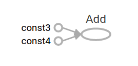 - -As it stands, this graph is not especially interesting because it always -produces a constant result. A graph can be parameterized to accept external -inputs, known as **placeholders**. A **placeholder** is a promise to provide a -value later. - -```python -a = tf.placeholder(tf.float32) -b = tf.placeholder(tf.float32) -adder_node = a + b # + provides a shortcut for tf.add(a, b) -``` - -The preceding three lines are a bit like a function or a lambda in which we -define two input parameters (a and b) and then an operation on them. We can -evaluate this graph with multiple inputs by using the feed_dict argument to -the [run method](https://www.tensorflow.org/api_docs/python/tf/Session#run) -to feed concrete values to the placeholders: - -```python -print(sess.run(adder_node, {a: 3, b: 4.5})) -print(sess.run(adder_node, {a: [1, 3], b: [2, 4]})) -``` -resulting in the output - -``` -7.5 -[ 3. 7.] -``` - -In TensorBoard, the graph looks like this: - -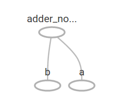 - -We can make the computational graph more complex by adding another operation. -For example, - -```python -add_and_triple = adder_node * 3. -print(sess.run(add_and_triple, {a: 3, b: 4.5})) -``` -produces the output -``` -22.5 -``` - -The preceding computational graph would look as follows in TensorBoard: - -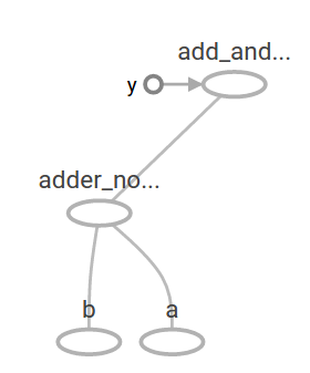 - -In machine learning we will typically want a model that can take arbitrary -inputs, such as the one above. To make the model trainable, we need to be able -to modify the graph to get new outputs with the same input. **Variables** allow -us to add trainable parameters to a graph. They are constructed with a type and -initial value: - - -```python -W = tf.Variable([.3], dtype=tf.float32) -b = tf.Variable([-.3], dtype=tf.float32) -x = tf.placeholder(tf.float32) -linear_model = W*x + b -``` - -Constants are initialized when you call `tf.constant`, and their value can never -change. By contrast, variables are not initialized when you call `tf.Variable`. -To initialize all the variables in a TensorFlow program, you must explicitly -call a special operation as follows: - -```python -init = tf.global_variables_initializer() -sess.run(init) -``` -It is important to realize `init` is a handle to the TensorFlow sub-graph that -initializes all the global variables. Until we call `sess.run`, the variables -are uninitialized. - - -Since `x` is a placeholder, we can evaluate `linear_model` for several values of -`x` simultaneously as follows: - -```python -print(sess.run(linear_model, {x: [1, 2, 3, 4]})) -``` -to produce the output -``` -[ 0. 0.30000001 0.60000002 0.90000004] -``` - -We've created a model, but we don't know how good it is yet. To evaluate the -model on training data, we need a `y` placeholder to provide the desired values, -and we need to write a loss function. - -A loss function measures how far apart the -current model is from the provided data. We'll use a standard loss model for -linear regression, which sums the squares of the deltas between the current -model and the provided data. `linear_model - y` creates a vector where each -element is the corresponding example's error delta. We call `tf.square` to -square that error. Then, we sum all the squared errors to create a single scalar -that abstracts the error of all examples using `tf.reduce_sum`: - -```python -y = tf.placeholder(tf.float32) -squared_deltas = tf.square(linear_model - y) -loss = tf.reduce_sum(squared_deltas) -print(sess.run(loss, {x: [1, 2, 3, 4], y: [0, -1, -2, -3]})) -``` -producing the loss value -``` -23.66 -``` - -We could improve this manually by reassigning the values of `W` and `b` to the -perfect values of -1 and 1. A variable is initialized to the value provided to -`tf.Variable` but can be changed using operations like `tf.assign`. For example, -`W=-1` and `b=1` are the optimal parameters for our model. We can change `W` and -`b` accordingly: - -```python -fixW = tf.assign(W, [-1.]) -fixb = tf.assign(b, [1.]) -sess.run([fixW, fixb]) -print(sess.run(loss, {x: [1, 2, 3, 4], y: [0, -1, -2, -3]})) -``` -The final print shows the loss now is zero. -``` -0.0 -``` - -We guessed the "perfect" values of `W` and `b`, but the whole point of machine -learning is to find the correct model parameters automatically. We will show -how to accomplish this in the next section. - -## tf.train API - -A complete discussion of machine learning is out of the scope of this tutorial. -However, TensorFlow provides **optimizers** that slowly change each variable in -order to minimize the loss function. The simplest optimizer is **gradient -descent**. It modifies each variable according to the magnitude of the -derivative of loss with respect to that variable. In general, computing symbolic -derivatives manually is tedious and error-prone. Consequently, TensorFlow can -automatically produce derivatives given only a description of the model using -the function `tf.gradients`. For simplicity, optimizers typically do this -for you. For example, - -```python -optimizer = tf.train.GradientDescentOptimizer(0.01) -train = optimizer.minimize(loss) -``` - -```python -sess.run(init) # reset variables to incorrect defaults. -for i in range(1000): - sess.run(train, {x: [1, 2, 3, 4], y: [0, -1, -2, -3]}) - -print(sess.run([W, b])) -``` -results in the final model parameters: -``` -[array([-0.9999969], dtype=float32), array([ 0.99999082], dtype=float32)] -``` - -Now we have done actual machine learning! Although this simple linear -regression model does not require much TensorFlow core code, more complicated -models and methods to feed data into your models necessitate more code. Thus, -TensorFlow provides higher level abstractions for common patterns, structures, -and functionality. We will learn how to use some of these abstractions in the -next section. - -### Complete program - -The completed trainable linear regression model is shown here: - -```python -import tensorflow as tf - -# Model parameters -W = tf.Variable([.3], dtype=tf.float32) -b = tf.Variable([-.3], dtype=tf.float32) -# Model input and output -x = tf.placeholder(tf.float32) -linear_model = W*x + b -y = tf.placeholder(tf.float32) - -# loss -loss = tf.reduce_sum(tf.square(linear_model - y)) # sum of the squares -# optimizer -optimizer = tf.train.GradientDescentOptimizer(0.01) -train = optimizer.minimize(loss) - -# training data -x_train = [1, 2, 3, 4] -y_train = [0, -1, -2, -3] -# training loop -init = tf.global_variables_initializer() -sess = tf.Session() -sess.run(init) # initialize variables with incorrect defaults. -for i in range(1000): - sess.run(train, {x: x_train, y: y_train}) - -# evaluate training accuracy -curr_W, curr_b, curr_loss = sess.run([W, b, loss], {x: x_train, y: y_train}) -print("W: %s b: %s loss: %s"%(curr_W, curr_b, curr_loss)) -``` -When run, it produces -``` -W: [-0.9999969] b: [ 0.99999082] loss: 5.69997e-11 -``` - -Notice that the loss is a very small number (very close to zero). If you run -this program, your loss may not be exactly the same as the aforementioned loss -because the model is initialized with pseudorandom values. - -This more complicated program can still be visualized in TensorBoard -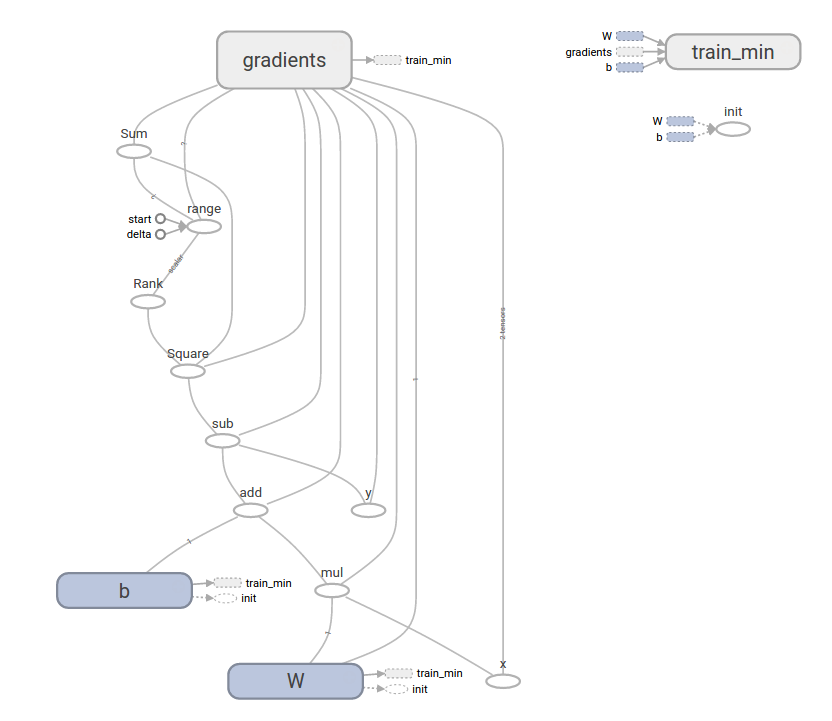 - -## `tf.estimator` - -`tf.estimator` is a high-level TensorFlow library that simplifies the -mechanics of machine learning, including the following: - -* running training loops -* running evaluation loops -* managing data sets - -tf.estimator defines many common models. - -### Basic usage - -Notice how much simpler the linear regression program becomes with -`tf.estimator`: - -```python -# NumPy is often used to load, manipulate and preprocess data. -import numpy as np -import tensorflow as tf - -# Declare list of features. We only have one numeric feature. There are many -# other types of columns that are more complicated and useful. -feature_columns = [tf.feature_column.numeric_column("x", shape=[1])] - -# An estimator is the front end to invoke training (fitting) and evaluation -# (inference). There are many predefined types like linear regression, -# linear classification, and many neural network classifiers and regressors. -# The following code provides an estimator that does linear regression. -estimator = tf.estimator.LinearRegressor(feature_columns=feature_columns) - -# TensorFlow provides many helper methods to read and set up data sets. -# Here we use two data sets: one for training and one for evaluation -# We have to tell the function how many batches -# of data (num_epochs) we want and how big each batch should be. -x_train = np.array([1., 2., 3., 4.]) -y_train = np.array([0., -1., -2., -3.]) -x_eval = np.array([2., 5., 8., 1.]) -y_eval = np.array([-1.01, -4.1, -7, 0.]) -input_fn = tf.estimator.inputs.numpy_input_fn( - {"x": x_train}, y_train, batch_size=4, num_epochs=None, shuffle=True) -train_input_fn = tf.estimator.inputs.numpy_input_fn( - {"x": x_train}, y_train, batch_size=4, num_epochs=1000, shuffle=False) -eval_input_fn = tf.estimator.inputs.numpy_input_fn( - {"x": x_eval}, y_eval, batch_size=4, num_epochs=1000, shuffle=False) - -# We can invoke 1000 training steps by invoking the method and passing the -# training data set. -estimator.train(input_fn=input_fn, steps=1000) - -# Here we evaluate how well our model did. -train_metrics = estimator.evaluate(input_fn=train_input_fn) -eval_metrics = estimator.evaluate(input_fn=eval_input_fn) -print("train metrics: %r"% train_metrics) -print("eval metrics: %r"% eval_metrics) -``` -When run, it produces something like -``` -train metrics: {'average_loss': 1.4833182e-08, 'global_step': 1000, 'loss': 5.9332727e-08} -eval metrics: {'average_loss': 0.0025353201, 'global_step': 1000, 'loss': 0.01014128} -``` -Notice how our eval data has a higher loss, but it is still close to zero. -That means we are learning properly. - -### A custom model - -`tf.estimator` does not lock you into its predefined models. Suppose we -wanted to create a custom model that is not built into TensorFlow. We can still -retain the high level abstraction of data set, feeding, training, etc. of -`tf.estimator`. For illustration, we will show how to implement our own -equivalent model to `LinearRegressor` using our knowledge of the lower level -TensorFlow API. - -To define a custom model that works with `tf.estimator`, we need to use -`tf.estimator.Estimator`. `tf.estimator.LinearRegressor` is actually -a sub-class of `tf.estimator.Estimator`. Instead of sub-classing -`Estimator`, we simply provide `Estimator` a function `model_fn` that tells -`tf.estimator` how it can evaluate predictions, training steps, and -loss. The code is as follows: - -```python -import numpy as np -import tensorflow as tf - -# Declare list of features, we only have one real-valued feature -def model_fn(features, labels, mode): - # Build a linear model and predict values - W = tf.get_variable("W", [1], dtype=tf.float64) - b = tf.get_variable("b", [1], dtype=tf.float64) - y = W*features['x'] + b - # Loss sub-graph - loss = tf.reduce_sum(tf.square(y - labels)) - # Training sub-graph - global_step = tf.train.get_global_step() - optimizer = tf.train.GradientDescentOptimizer(0.01) - train = tf.group(optimizer.minimize(loss), - tf.assign_add(global_step, 1)) - # EstimatorSpec connects subgraphs we built to the - # appropriate functionality. - return tf.estimator.EstimatorSpec( - mode=mode, - predictions=y, - loss=loss, - train_op=train) - -estimator = tf.estimator.Estimator(model_fn=model_fn) -# define our data sets -x_train = np.array([1., 2., 3., 4.]) -y_train = np.array([0., -1., -2., -3.]) -x_eval = np.array([2., 5., 8., 1.]) -y_eval = np.array([-1.01, -4.1, -7., 0.]) -input_fn = tf.estimator.inputs.numpy_input_fn( - {"x": x_train}, y_train, batch_size=4, num_epochs=None, shuffle=True) -train_input_fn = tf.estimator.inputs.numpy_input_fn( - {"x": x_train}, y_train, batch_size=4, num_epochs=1000, shuffle=False) -eval_input_fn = tf.estimator.inputs.numpy_input_fn( - {"x": x_eval}, y_eval, batch_size=4, num_epochs=1, shuffle=False) - -# train -estimator.train(input_fn=input_fn, steps=1000) -# Here we evaluate how well our model did. -train_metrics = estimator.evaluate(input_fn=train_input_fn) -eval_metrics = estimator.evaluate(input_fn=eval_input_fn) -print("train metrics: %r"% train_metrics) -print("eval metrics: %r"% eval_metrics) -``` -When run, it produces -``` -train metrics: {'loss': 1.227995e-11, 'global_step': 1000} -eval metrics: {'loss': 0.01010036, 'global_step': 1000} -``` - -Notice how the contents of the custom `model_fn()` function are very similar -to our manual model training loop from the lower level API. - -## Next steps - -Now you have a working knowledge of the basics of TensorFlow. We have several -more tutorials that you can look at to learn more. If you are a beginner in -machine learning see @{$beginners$MNIST for beginners}, -otherwise see @{$pros$Deep MNIST for experts}. diff --git a/tensorflow/docs_src/get_started/get_started_for_beginners.md b/tensorflow/docs_src/get_started/get_started_for_beginners.md new file mode 100644 index 0000000000..ea1c2fb3f4 --- /dev/null +++ b/tensorflow/docs_src/get_started/get_started_for_beginners.md @@ -0,0 +1,732 @@ +# Getting Started for ML Beginners + +This document explains how to use machine learning to classify (categorize) +Iris flowers by species. This document dives deeply into the TensorFlow +code to do exactly that, explaining ML fundamentals along the way. + +If the following list describes you, then you are in the right place: + +* You know little to nothing about machine learning. +* You want to learn how to write TensorFlow programs. +* You can code (at least a little) in Python. + +If you are already familiar with basic machine learning concepts +but are new to TensorFlow, read +@{$premade_estimators$Getting Started with TensorFlow: for ML Experts}. + +## The Iris classification problem + +Imagine you are a botanist seeking an automated way to classify each +Iris flower you find. Machine learning provides many ways to classify flowers. +For instance, a sophisticated machine learning program could classify flowers +based on photographs. Our ambitions are more modest--we're going to classify +Iris flowers based solely on the length and width of their +[sepals](https://en.wikipedia.org/wiki/Sepal) and +[petals](https://en.wikipedia.org/wiki/Petal). + +The Iris genus entails about 300 species, but our program will classify only +the following three: + +* Iris setosa +* Iris virginica +* Iris versicolor + +<div style="margin:auto; margin-bottom:10px; margin-top:20px;"> +<img style="width:100%" + alt="Petal geometry compared for three iris species: Iris setosa, Iris virginica, and Iris versicolor" + src="../images/iris_three_species.jpg"> +</div> +**From left to right, +[*Iris setosa*](https://commons.wikimedia.org/w/index.php?curid=170298) (by +[Radomil](https://commons.wikimedia.org/wiki/User:Radomil), CC BY-SA 3.0), +[*Iris versicolor*](https://commons.wikimedia.org/w/index.php?curid=248095) (by +[Dlanglois](https://commons.wikimedia.org/wiki/User:Dlanglois), CC BY-SA 3.0), +and [*Iris virginica*](https://www.flickr.com/photos/33397993@N05/3352169862) +(by [Frank Mayfield](https://www.flickr.com/photos/33397993@N05), CC BY-SA +2.0).** +<p> </p> + +Fortunately, someone has already created [a data set of 120 Iris +flowers](https://en.wikipedia.org/wiki/Iris_flower_data_set) +with the sepal and petal measurements. This data set has become +one of the canonical introductions to machine learning classification problems. +(The [MNIST database](https://en.wikipedia.org/wiki/MNIST_database), +which contains handwritten digits, is another popular classification +problem.) The first 5 entries of the Iris data set +look as follows: + +| Sepal length | sepal width | petal length | petal width | species +| --- | --- | --- | --- | --- +|6.4 | 2.8 | 5.6 | 2.2 | 2 +|5.0 | 2.3 | 3.3 | 1.0 | 1 +|4.9 | 2.5 | 4.5 | 1.7 | 2 +|4.9 | 3.1 | 1.5 | 0.1 | 0 +|5.7 | 3.8 | 1.7 | 0.3 | 0 + +Let's introduce some terms: + +* The last column (species) is called the + [**label**](https://developers.google.com/machine-learning/glossary/#label); + the first four columns are called + [**features**](https://developers.google.com/machine-learning/glossary/#feature). + Features are characteristics of an example, while the label is + the thing we're trying to predict. + +* An [**example**](https://developers.google.com/machine-learning/glossary/#example) + consists of the set of features and the label for one sample + flower. The preceding table shows 5 examples from a data set of + 120 examples. + +Each label is naturally a string (for example, "setosa"), but machine learning +typically relies on numeric values. Therefore, someone mapped each string to +a number. Here's the representation scheme: + +* 0 represents setosa +* 1 represents versicolor +* 2 represents virginica + + +## Models and training + +A **model** is the relationship between features +and the label. For the Iris problem, the model defines the relationship +between the sepal and petal measurements and the Iris species. +Some simple models can be described with a few lines of algebra; +more complex machine learning models +contain such a large number of interlacing mathematical functions and +parameters that they become hard to summarize mathematically. + +Could you determine the relationship between the four features and the +Iris species *without* using machine learning? That is, could you use +traditional programming techniques (for example, a lot of conditional +statements) to create a model? Maybe. You could play with the data set +long enough to determine the right relationships of petal and sepal +measurements to particular species. However, a good machine learning +approach *determines the model for you*. That is, if you feed enough +representative examples into the right machine learning model type, the program +will determine the relationship between sepals, petals, and species. + +**Training** is the stage of machine learning in which the model is +gradually optimized (learned). The Iris problem is an example +of [**supervised machine +learning**](https://developers.google.com/machine-learning/glossary/#supervised_machine_learning) +in which a model is trained from examples that contain labels. (In +[**unsupervised machine +learning**](https://developers.google.com/machine-learning/glossary/#unsupervised_machine_learning), +the examples don't contain labels. Instead, the model typically finds +patterns among the features.) + + + + +## Get the sample program + +Prior to playing with the sample code in this document, do the following: + +1. @{$install$Install TensorFlow}. +2. If you installed TensorFlow with virtualenv or Anaconda, activate your + TensorFlow environment. +3. Install or upgrade pandas by issuing the following command: + + `pip install pandas` + + +Take the following steps to get the sample program: + +1. Clone the TensorFlow Models repository from github by entering the following + command: + + `git clone https://github.com/tensorflow/models` + +2. Change directory within that branch to the location containing the examples + used in this document: + + `cd models/samples/core/get_started/` + +In that `get_started` directory, you'll find a program +named `premade_estimator.py`. + + +## Run the sample program + +You run TensorFlow programs as you would run any Python program. Therefore, +issue the following command from a command line to +run `premade_estimators.py`: + +``` bash +python premade_estimator.py +``` + +Running the program should output a whole bunch of information ending with +three prediction lines like the following: + +```None +... +Prediction is "Setosa" (99.6%), expected "Setosa" + +Prediction is "Versicolor" (99.8%), expected "Versicolor" + +Prediction is "Virginica" (97.9%), expected "Virginica" +``` + +If the program generates errors instead of predictions, ask yourself the +following questions: + +* Did you install TensorFlow properly? +* Are you using the correct version of TensorFlow? The `premade_estimators.py` + program requires at least TensorFlow v1.4. +* If you installed TensorFlow with virtualenv or Anaconda, did you activate + the environment? + + + +## The TensorFlow programming stack + +As the following illustration shows, TensorFlow +provides a programming stack consisting of multiple API layers: + +<div style="margin:auto; margin-bottom:10px; margin-top:20px;"> +<img style="width:100%" src="../images/tensorflow_programming_environment.png"> +</div> +**The TensorFlow Programming Environment.** +<p> </p> + +As you start writing TensorFlow programs, we strongly recommend focusing on +the following two high-level APIs: + +* Estimators +* Datasets + +Although we'll grab an occasional convenience function from other APIs, +this document focuses on the preceding two APIs. + + +## The program itself + +Thanks for your patience; let's dig into the code. +The general outline of `premade_estimator.py`--and many other TensorFlow +programs--is as follows: + +* Import and parse the data sets. +* Create feature columns to describe the data. +* Select the type of model +* Train the model. +* Evaluate the model's effectiveness. +* Let the trained model make predictions. + +The following subsections detail each part. + + +### Import and parse the data sets + +The Iris program requires the data from the following two .csv files: + +* `http://download.tensorflow.org/data/iris_training.csv`, which contains + the training set. +* `http://download.tensorflow.org/data/iris_test.csv`, which contains the + the test set. + +The **training set** contains the examples that we'll use to train the model; +the **test set** contains the examples that we'll use to evaluate the trained +model's effectiveness. + +The training set and test set started out as a +single data set. Then, someone split the examples, with the majority going into +the training set and the remainder going into the test set. Adding +examples to the training set usually builds a better model; however, adding +more examples to the test set enables us to better gauge the model's +effectiveness. Regardless of the split, the examples in the test set +must be separate from the examples in the training set. Otherwise, you can't +accurately determine the model's effectiveness. + +The `premade_estimators.py` program relies on the `load_data` function +in the adjacent [`iris_data.py`]( +https://github.com/tensorflow/models/blob/master/samples/core/get_started/iris_data.py) +file to read in and parse the training set and test set. +Here is a heavily commented version of the function: + +```python +TRAIN_URL = "http://download.tensorflow.org/data/iris_training.csv" +TEST_URL = "http://download.tensorflow.org/data/iris_test.csv" + +CSV_COLUMN_NAMES = ['SepalLength', 'SepalWidth', + 'PetalLength', 'PetalWidth', 'Species'] + +... + +def load_data(label_name='Species'): + """Parses the csv file in TRAIN_URL and TEST_URL.""" + + # Create a local copy of the training set. + train_path = tf.keras.utils.get_file(fname=TRAIN_URL.split('/')[-1], + origin=TRAIN_URL) + # train_path now holds the pathname: ~/.keras/datasets/iris_training.csv + + # Parse the local CSV file. + train = pd.read_csv(filepath_or_buffer=train_path, + names=CSV_COLUMN_NAMES, # list of column names + header=0 # ignore the first row of the CSV file. + ) + # train now holds a pandas DataFrame, which is data structure + # analogous to a table. + + # 1. Assign the DataFrame's labels (the right-most column) to train_label. + # 2. Delete (pop) the labels from the DataFrame. + # 3. Assign the remainder of the DataFrame to train_features + train_features, train_label = train, train.pop(label_name) + + # Apply the preceding logic to the test set. + test_path = tf.keras.utils.get_file(TEST_URL.split('/')[-1], TEST_URL) + test = pd.read_csv(test_path, names=CSV_COLUMN_NAMES, header=0) + test_features, test_label = test, test.pop(label_name) + + # Return four DataFrames. + return (train_features, train_label), (test_features, test_label) +``` + +Keras is an open-sourced machine learning library; `tf.keras` is a TensorFlow +implementation of Keras. The `premade_estimator.py` program only accesses +one `tf.keras` function; namely, the `tf.keras.utils.get_file` convenience +function, which copies a remote CSV file to a local file system. + +The call to `load_data` returns two `(feature,label)` pairs, for the training +and test sets respectively: + +```python + # Call load_data() to parse the CSV file. + (train_feature, train_label), (test_feature, test_label) = load_data() +``` + +Pandas is an open-source Python library leveraged by several +TensorFlow functions. A pandas +[**DataFrame**](https://pandas.pydata.org/pandas-docs/stable/generated/pandas.DataFrame.html) +is a table with named columns headers and numbered rows. +The features returned by `load_data` are packed in `DataFrames`. +For example, the `test_feature` DataFrame looks as follows: + +```none + SepalLength SepalWidth PetalLength PetalWidth +0 5.9 3.0 4.2 1.5 +1 6.9 3.1 5.4 2.1 +2 5.1 3.3 1.7 0.5 +... +27 6.7 3.1 4.7 1.5 +28 6.7 3.3 5.7 2.5 +29 6.4 2.9 4.3 1.3 +``` + + +### Describe the data + +A **feature column** is a data structure that tells your model +how to interpret the data in each feature. In the Iris problem, +we want the model to interpret the data in each +feature as its literal floating-point value; that is, we want the +model to interpret an input value like 5.4 as, well, 5.4. However, +in other machine learning problems, it is often desirable to interpret +data less literally. Using feature columns to +interpret data is such a rich topic that we devote an entire +@{$feature_columns$document} to it. + +From a code perspective, you build a list of `feature_column` objects by calling +functions from the @{tf.feature_column} module. Each object describes an input +to the model. To tell the model to interpret data as a floating-point value, +call @{tf.feature_column.numeric_column). In `premade_estimator.py`, all +four features should be interpreted as literal floating-point values, so +the code to create a feature column looks as follows: + +```python +# Create feature columns for all features. +my_feature_columns = [] +for key in train_x.keys(): + my_feature_columns.append(tf.feature_column.numeric_column(key=key)) +``` + +Here is a less elegant, but possibly clearer, alternative way to +encode the preceding block: + +```python +my_feature_columns = [ + tf.feature_column.numeric_column(key='SepalLength'), + tf.feature_column.numeric_column(key='SepalWidth'), + tf.feature_column.numeric_column(key='PetalLength'), + tf.feature_column.numeric_column(key='PetalWidth') +] +``` + + +### Select the type of model + +We need the select the kind of model that will be trained. +Lots of model types exist; picking the ideal type takes experience. +We've selected a neural network to solve the Iris problem. [**Neural +networks**](https://developers.google.com/machine-learning/glossary/#neural_network) +can find complex relationships between features and the label. +A neural network is a highly-structured graph, organized into one or more +[**hidden layers**](https://developers.google.com/machine-learning/glossary/#hidden_layer). +Each hidden layer consists of one or more +[**neurons**](https://developers.google.com/machine-learning/glossary/#neuron). +There are several categories of neural networks. +We'll be using a [**fully connected neural +network**](https://developers.google.com/machine-learning/glossary/#fully_connected_layer), +which means that the neurons in one layer take inputs from *every* neuron in +the previous layer. For example, the following figure illustrates a +fully connected neural network consisting of three hidden layers: + +* The first hidden layer contains four neurons. +* The second hidden layer contains three neurons. +* The third hidden layer contains two neurons. + +<div style="margin:auto; margin-bottom:10px; margin-top:20px;"> +<img style="width:100%" src="../images/simple_dnn.svg"> +</div> +**A neural network with three hidden layers.** +<p> </p> + +To specify a model type, instantiate an +[**Estimator**](https://developers.google.com/machine-learning/glossary/#Estimators) +class. TensorFlow provides two categories of Estimators: + +* [**pre-made + Estimators**](https://developers.google.com/machine-learning/glossary/#pre-made_Estimator), + which someone else has already written for you. +* [**custom + Estimators**](https://developers.google.com/machine-learning/glossary/#custom_estimator), + which you must code yourself, at least partially. + +To implement a neural network, the `premade_estimators.py` program uses +a pre-made Estimator named @{tf.estimator.DNNClassifier}. This Estimator +builds a neural network that classifies examples. The following call +instantiates `DNNClassifier`: + +```python + classifier = tf.estimator.DNNClassifier( + feature_columns=my_feature_columns, + hidden_units=[10, 10], + n_classes=3) +``` + +Use the `hidden_units` parameter to define the number of neurons +in each hidden layer of the neural network. Assign this parameter +a list. For example: + +```python + hidden_units=[10, 10], +``` + +The length of the list assigned to `hidden_units` identifies the number of +hidden layers (2, in this case). +Each value in the list represents the number of neurons in a particular +hidden layer (10 in the first hidden layer and 10 in the second hidden layer). +To change the number of hidden layers or neurons, simply assign a different +list to the `hidden_units` parameter. + +The ideal number of hidden layers and neurons depends on the problem +and the data set. Like many aspects of machine learning, +picking the ideal shape of the neural network requires some mixture +of knowledge and experimentation. +As a rule of thumb, increasing the number of hidden layers and neurons +*typically* creates a more powerful model, which requires more data to +train effectively. + +The `n_classes` parameter specifies the number of possible values that the +neural network can predict. Since the Iris problem classifies 3 Iris species, +we set `n_classes` to 3. + +The constructor for `tf.Estimator.DNNClassifier` takes an optional argument +named `optimizer`, which our sample code chose not to specify. The +[**optimizer**](https://developers.google.com/machine-learning/glossary/#optimizer) +controls how the model will train. As you develop more expertise in machine +learning, optimizers and +[**learning +rate**](https://developers.google.com/machine-learning/glossary/#learning_rate) +will become very important. + + + +### Train the model + +Instantiating a `tf.Estimator.DNNClassifier` creates a framework for learning +the model. Basically, we've wired a network but haven't yet let data flow +through it. To train the neural network, call the Estimator object's `train` +method. For example: + +```python + classifier.train( + input_fn=lambda:train_input_fn(train_feature, train_label, args.batch_size), + steps=args.train_steps) +``` + +The `steps` argument tells `train` to stop training after the specified +number of iterations. Increasing `steps` increases the amount of time +the model will train. Counter-intuitively, training a model longer +does not guarantee a better model. The default value of `args.train_steps` +is 1000. The number of steps to train is a +[**hyperparameter**](https://developers.google.com/machine-learning/glossary/#hyperparameter) +you can tune. Choosing the right number of steps usually +requires both experience and experimentation. + +The `input_fn` parameter identifies the function that supplies the +training data. The call to the `train` method indicates that the +`train_input_fn` function will supply the training data. Here's that +method's signature: + +```python +def train_input_fn(features, labels, batch_size): +``` + +We're passing the following arguments to `train_input_fn`: + +* `train_feature` is a Python dictionary in which: + * Each key is the name of a feature. + * Each value is an array containing the values for each example in the + training set. +* `train_label` is an array containing the values of the label for every + example in the training set. +* `args.batch_size` is an integer defining the [**batch + size**](https://developers.google.com/machine-learning/glossary/#batch_size). + +The `train_input_fn` function relies on the **Dataset API**. This is a +high-level TensorFlow API for reading data and transforming it into a form +that the `train` method requires. The following call converts the +input features and labels into a `tf.data.Dataset` object, which is the base +class of the Dataset API: + +```python + dataset = tf.data.Dataset.from_tensor_slices((dict(features), labels)) +``` + +The `tf.dataset` class provides many useful functions for preparing examples +for training. The following line calls three of those functions: + +```python + dataset = dataset.shuffle(buffer_size=1000).repeat(count=None).batch(batch_size) +``` + +Training works best if the training examples are in +random order. To randomize the examples, call +`tf.data.Dataset.shuffle`. Setting the `buffer_size` to a value +larger than the number of examples (120) ensures that the data will +be well shuffled. + +During training, the `train` method typically processes the +examples multiple times. Calling the +`tf.data.Dataset.repeat` method without any arguments ensures +that the `train` method has an infinite supply of (now shuffled) +training set examples. + +The `train` method processes a +[**batch**](https://developers.google.com/machine-learning/glossary/#batch) +of examples at a time. +The `tf.data.Dataset.batch` method creates a batch by +concatenating multiple examples. +This program sets the default [**batch +size**](https://developers.google.com/machine-learning/glossary/#batch_size) +to 100, meaning that the `batch` method will concatenate groups of +100 examples. The ideal batch size depends on the problem. As a rule +of thumb, smaller batch sizes usually enable the `train` method to train +the model faster at the expense (sometimes) of accuracy. + +The following `return` statement passes a batch of examples back to +the caller (the `train` method). + +```python + return dataset.make_one_shot_iterator().get_next() +``` + + +### Evaluate the model + +**Evaluating** means determining how effectively the model makes +predictions. To determine the Iris classification model's effectiveness, +pass some sepal and petal measurements to the model and ask the model +to predict what Iris species they represent. Then compare the model's +prediction against the actual label. For example, a model that picked +the correct species on half the input examples would have an +[accuracy](https://developers.google.com/machine-learning/glossary/#accuracy) +of 0.5. The following suggests a more effective model: + + +<table> + <tr> + <th style="background-color:darkblue" colspan="5"> + Test Set</th> + </tr> + <tr> + <th colspan="4">Features</th> + <th colspan="1">Label</th> + <th colspan="1">Prediction</th> + </tr> + <tr> <td>5.9</td> <td>3.0</td> <td>4.3</td> <td>1.5</td> <td>1</td> + <td style="background-color:green">1</td></tr> + <tr> <td>6.9</td> <td>3.1</td> <td>5.4</td> <td>2.1</td> <td>2</td> + <td style="background-color:green">2</td></tr> + <tr> <td>5.1</td> <td>3.3</td> <td>1.7</td> <td>0.5</td> <td>0</td> + <td style="background-color:green">0</td></tr> + <tr> <td>6.0</td> <td>3.4</td> <td>4.5</td> <td>1.6</td> <td>1</td> + <td style="background-color:red">2</td></tr> + <tr> <td>5.5</td> <td>2.5</td> <td>4.0</td> <td>1.3</td> <td>1</td> + <td style="background-color:green">1</td></tr> +</table> +**A model that is 80% accurate.** +<p> </p> + +To evaluate a model's effectiveness, each Estimator provides an `evaluate` +method. The `premade_estimator.py` program calls `evaluate` as follows: + +```python +# Evaluate the model. +eval_result = classifier.evaluate( + input_fn=lambda:eval_input_fn(test_x, test_y, args.batch_size)) + +print('\nTest set accuracy: {accuracy:0.3f}\n'.format(**eval_result)) +``` + +The call to `classifier.evaluate` is similar to the call to `classifier.train`. +The biggest difference is that `classifier.evaluate` must get its examples +from the test set rather than the training set. In other words, to +fairly assess a model's effectiveness, the examples used to +*evaluate* a model must be different from the examples used to *train* +the model. The `eval_input_fn` function serves a batch of examples from +the test set. Here's the `eval_input_fn` method: + +```python +def eval_input_fn(features, labels=None, batch_size=None): + """An input function for evaluation or prediction""" + if labels is None: + # No labels, use only features. + inputs = features + else: + inputs = (features, labels) + + # Convert inputs to a tf.dataset object. + dataset = tf.data.Dataset.from_tensor_slices(inputs) + + # Batch the examples + assert batch_size is not None, "batch_size must not be None" + dataset = dataset.batch(batch_size) + + # Return the read end of the pipeline. + return dataset.make_one_shot_iterator().get_next() +``` + +In brief, `eval_input_fn` does the following when called by +`classifier.evaluate`: + +1. Converts the features and labels from the test set to a `tf.dataset` + object. +2. Creates a batch of test set examples. (There's no need to shuffle + or repeat the test set examples.) +3. Returns that batch of test set examples to `classifier.evaluate`. + +Running this code yields the following output (or something close to it): + +```none +Test set accuracy: 0.967 +``` + +An accuracy of 0.967 implies that our trained model correctly classified 29 +out of the 30 Iris species in the test set. + + +### Predicting + +We've now trained a model and "proven" that it is good--but not +perfect--at classifying Iris species. Now let's use the trained +model to make some predictions on [**unlabeled +examples**](https://developers.google.com/machine-learning/glossary/#unlabeled_example); +that is, on examples that contain features but not a label. + +In real-life, the unlabeled examples could come from lots of different +sources including apps, CSV files, and data feeds. For now, we're simply +going to manually provide the following three unlabeled examples: + +```python + predict_x = { + 'SepalLength': [5.1, 5.9, 6.9], + 'SepalWidth': [3.3, 3.0, 3.1], + 'PetalLength': [1.7, 4.2, 5.4], + 'PetalWidth': [0.5, 1.5, 2.1], + } +``` + +Every Estimator provides a `predict` method, which `premade_estimator.py` +calls as follows: + +```python +predictions = classifier.predict( + input_fn=lambda:eval_input_fn(predict_x, batch_size=args.batch_size)) +``` + +As with the `evaluate` method, our `predict` method also gathers examples +from the `eval_input_fn` method. + +When doing predictions, we're *not* passing labels to `eval_input_fn`. +Therefore, `eval_input_fn` does the following: + +1. Converts the features from the 3-element manual set we just created. +2. Creates a batch of 3 examples from that manual set. +3. Returns that batch of examples to `classifier.predict`. + +The `predict` method returns a python iterable, yielding a dictionary of +prediction results for each example. This dictionary contains several keys. +The `probabilities` key holds a list of three floating-point values, +each representing the probability that the input example is a particular +Iris species. For example, consider the following `probabilities` list: + +```none +'probabilities': array([ 1.19127117e-08, 3.97069454e-02, 9.60292995e-01]) +``` + +The preceding list indicates: + +* A negligible chance of the Iris being Setosa. +* A 3.97% chance of the Iris being Versicolor. +* A 96.0% chance of the Iris being Virginica. + +The `class_ids` key holds a one-element array that identifies the most +probable species. For example: + +```none +'class_ids': array([2]) +``` + +The number `2` corresponds to Virginica. The following code iterates +through the returned `predictions` to report on each prediction: + +``` python +for pred_dict, expec in zip(predictions, expected): + template = ('\nPrediction is "{}" ({:.1f}%), expected "{}"') + + class_id = pred_dict['class_ids'][0] + probability = pred_dict['probabilities'][class_id] + print(template.format(SPECIES[class_id], 100 * probability, expec)) +``` + +Running the program yields the following output: + + +``` None +... +Prediction is "Setosa" (99.6%), expected "Setosa" + +Prediction is "Versicolor" (99.8%), expected "Versicolor" + +Prediction is "Virginica" (97.9%), expected "Virginica" +``` + + +## Summary + +<!--TODO(barryr): When MLCC is released, add pointers to relevant sections.--> +This document provides a short introduction to machine learning. + +Because `premade_estimators.py` relies on high-level APIs, much of the +mathematical complexity in machine learning is hidden. +If you intend to become more proficient in machine learning, we recommend +ultimately learning more about [**gradient +descent**](https://developers.google.com/machine-learning/glossary/#gradient_descent), +batching, and neural networks. + +We recommend reading the @{$feature_columns$Feature Columns} document next, +which explains how to represent different kinds of data in machine learning. diff --git a/tensorflow/docs_src/get_started/index.md b/tensorflow/docs_src/get_started/index.md index 003fac1a28..d0cb69d211 100644 --- a/tensorflow/docs_src/get_started/index.md +++ b/tensorflow/docs_src/get_started/index.md @@ -1,36 +1,35 @@ # Getting Started -For a brief overview of TensorFlow programming fundamentals, see the following -guide: - - * @{$get_started/get_started$Getting Started with TensorFlow} - -MNIST has become the canonical dataset for trying out a new machine learning -toolkit. We offer three guides that each demonstrate a different approach -to training an MNIST model on TensorFlow: - - * @{$mnist/beginners$MNIST for ML Beginners}, which introduces MNIST through - the high-level API. - * @{$mnist/pros$Deep MNIST for Experts}, which is more-in depth than - "MNIST for ML Beginners," and assumes some familiarity with machine - learning concepts. - * @{$mnist/mechanics$TensorFlow Mechanics 101}, which introduces MNIST through - the low-level API. - -For developers new to TensorFlow, the high-level API is a good place to start. -To learn about the high-level API, read the following guides: - - * @{$get_started/estimator$tf.estimator Quickstart}, which introduces this - API. - * @{$get_started/input_fn$Building Input Functions}, - which takes you into a somewhat more sophisticated use of this API. - -TensorBoard is a utility to visualize different aspects of machine learning. -The following guides explain how to use TensorBoard: - - * @{$get_started/summaries_and_tensorboard$TensorBoard: Visualizing Learning}, - which gets you started. - * @{$get_started/graph_viz$TensorBoard: Graph Visualization}, which explains - how to visualize the computational graph. Graph visualization is typically - more useful for programmers using the low-level API. - +TensorFlow is a tool for machine learning. While it contains a wide range of +functionality, it is mainly designed for deep neural network models. + +The fastest way to build a fully-featured model trained on your data is to use +TensorFlow's high-level API. In the following examples, we will use the +high-level API on the classic [Iris dataset](https://en.wikipedia.org/wiki/Iris_flower_data_set). +We will train a model that predicts what species a flower is based on its +characteristics, and along the way get a quick introduction to the basic tasks +in TensorFlow using Estimators. + +This tutorial is divided into the following parts: + + * @{$get_started/premade_estimators}, which shows you + how to quickly setup prebuilt models to train on in-memory data. + * @{$get_started/checkpoints}, which shows you how to save training progress, + and resume where you left off. + * @{$get_started/feature_columns}, which shows how an + Estimator can handle a variety of input data types without changes to the + model. + * @{$get_started/datasets_quickstart}, which is a minimal introduction to + the TensorFlow's input pipelines. + * @{$get_started/custom_estimators}, which demonstrates how + to build and train models you design yourself. + +For more advanced users: + + * The @{$low_level_intro$Low Level Introduction} demonstrates how to use + tensorflow outside of the Estimator framework, for debugging and + experimentation. + * The remainder of the @{$programmers_guide$Programmer's Guide} contains + in-depth guides to various major components of TensorFlow. + * The @{$tutorials$Tutorials} provide walkthroughs of a variety of + TensorFlow models. diff --git a/tensorflow/docs_src/get_started/input_fn.md b/tensorflow/docs_src/get_started/input_fn.md deleted file mode 100644 index 24bfdbdd2e..0000000000 --- a/tensorflow/docs_src/get_started/input_fn.md +++ /dev/null @@ -1,438 +0,0 @@ -# Building Input Functions with tf.estimator - -This tutorial introduces you to creating input functions in tf.estimator. -You'll get an overview of how to construct an `input_fn` to preprocess and feed -data into your models. Then, you'll implement an `input_fn` that feeds training, -evaluation, and prediction data into a neural network regressor for predicting -median house values. - -## Custom Input Pipelines with input_fn - -The `input_fn` is used to pass feature and target data to the `train`, -`evaluate`, and `predict` methods of the `Estimator`. -The user can do feature engineering or pre-processing inside the `input_fn`. -Here's an example taken from the @{$get_started/estimator$tf.estimator Quickstart tutorial}: - -```python -import numpy as np - -training_set = tf.contrib.learn.datasets.base.load_csv_with_header( - filename=IRIS_TRAINING, target_dtype=np.int, features_dtype=np.float32) - -train_input_fn = tf.estimator.inputs.numpy_input_fn( - x={"x": np.array(training_set.data)}, - y=np.array(training_set.target), - num_epochs=None, - shuffle=True) - -classifier.train(input_fn=train_input_fn, steps=2000) -``` - -### Anatomy of an input_fn - -The following code illustrates the basic skeleton for an input function: - -```python -def my_input_fn(): - - # Preprocess your data here... - - # ...then return 1) a mapping of feature columns to Tensors with - # the corresponding feature data, and 2) a Tensor containing labels - return feature_cols, labels -``` - -The body of the input function contains the specific logic for preprocessing -your input data, such as scrubbing out bad examples or -[feature scaling](https://en.wikipedia.org/wiki/Feature_scaling). - -Input functions must return the following two values containing the final -feature and label data to be fed into your model (as shown in the above code -skeleton): - -<dl> - <dt><code>feature_cols</code></dt> - <dd>A dict containing key/value pairs that map feature column -names to <code>Tensor</code>s (or <code>SparseTensor</code>s) containing the corresponding feature -data.</dd> - <dt><code>labels</code></dt> - <dd>A <code>Tensor</code> containing your label (target) values: the values your model aims to predict.</dd> -</dl> - -### Converting Feature Data to Tensors - -If your feature/label data is a python array or stored in -[_pandas_](http://pandas.pydata.org/) dataframes or -[numpy](http://www.numpy.org/) arrays, you can use the following methods to -construct `input_fn`: - -```python -import numpy as np -# numpy input_fn. -my_input_fn = tf.estimator.inputs.numpy_input_fn( - x={"x": np.array(x_data)}, - y=np.array(y_data), - ...) -``` - -```python -import pandas as pd -# pandas input_fn. -my_input_fn = tf.estimator.inputs.pandas_input_fn( - x=pd.DataFrame({"x": x_data}), - y=pd.Series(y_data), - ...) -``` - -For [sparse, categorical data](https://en.wikipedia.org/wiki/Sparse_matrix) -(data where the majority of values are 0), you'll instead want to populate a -`SparseTensor`, which is instantiated with three arguments: - -<dl> - <dt><code>dense_shape</code></dt> - <dd>The shape of the tensor. Takes a list indicating the number of elements in each dimension. For example, <code>dense_shape=[3,6]</code> specifies a two-dimensional 3x6 tensor, <code>dense_shape=[2,3,4]</code> specifies a three-dimensional 2x3x4 tensor, and <code>dense_shape=[9]</code> specifies a one-dimensional tensor with 9 elements.</dd> - <dt><code>indices</code></dt> - <dd>The indices of the elements in your tensor that contain nonzero values. Takes a list of terms, where each term is itself a list containing the index of a nonzero element. (Elements are zero-indexed—i.e., [0,0] is the index value for the element in the first column of the first row in a two-dimensional tensor.) For example, <code>indices=[[1,3], [2,4]]</code> specifies that the elements with indexes of [1,3] and [2,4] have nonzero values.</dd> - <dt><code>values</code></dt> - <dd>A one-dimensional tensor of values. Term <code>i</code> in <code>values</code> corresponds to term <code>i</code> in <code>indices</code> and specifies its value. For example, given <code>indices=[[1,3], [2,4]]</code>, the parameter <code>values=[18, 3.6]</code> specifies that element [1,3] of the tensor has a value of 18, and element [2,4] of the tensor has a value of 3.6.</dd> -</dl> - -The following code defines a two-dimensional `SparseTensor` with 3 rows and 5 -columns. The element with index [0,1] has a value of 6, and the element with -index [2,4] has a value of 0.5 (all other values are 0): - -```python -sparse_tensor = tf.SparseTensor(indices=[[0,1], [2,4]], - values=[6, 0.5], - dense_shape=[3, 5]) -``` - -This corresponds to the following dense tensor: - -```none -[[0, 6, 0, 0, 0] - [0, 0, 0, 0, 0] - [0, 0, 0, 0, 0.5]] -``` - -For more on `SparseTensor`, see @{tf.SparseTensor}. - -### Passing input_fn Data to Your Model - -To feed data to your model for training, you simply pass the input function -you've created to your `train` operation as the value of the `input_fn` -parameter, e.g.: - -```python -classifier.train(input_fn=my_input_fn, steps=2000) -``` - -Note that the `input_fn` parameter must receive a function object (i.e., -`input_fn=my_input_fn`), not the return value of a function call -(`input_fn=my_input_fn()`). This means that if you try to pass parameters to the -`input_fn` in your `train` call, as in the following code, it will result in a -`TypeError`: - -```python -classifier.train(input_fn=my_input_fn(training_set), steps=2000) -``` - -However, if you'd like to be able to parameterize your input function, there are -other methods for doing so. You can employ a wrapper function that takes no -arguments as your `input_fn` and use it to invoke your input function -with the desired parameters. For example: - -```python -def my_input_fn(data_set): - ... - -def my_input_fn_training_set(): - return my_input_fn(training_set) - -classifier.train(input_fn=my_input_fn_training_set, steps=2000) -``` - -Alternatively, you can use Python's [`functools.partial`](https://docs.python.org/2/library/functools.html#functools.partial) -function to construct a new function object with all parameter values fixed: - -```python -classifier.train( - input_fn=functools.partial(my_input_fn, data_set=training_set), - steps=2000) -``` - -A third option is to wrap your `input_fn` invocation in a -[`lambda`](https://docs.python.org/3/tutorial/controlflow.html#lambda-expressions) -and pass it to the `input_fn` parameter: - -```python -classifier.train(input_fn=lambda: my_input_fn(training_set), steps=2000) -``` - -One big advantage of designing your input pipeline as shown above—to accept a -parameter for data set—is that you can pass the same `input_fn` to `evaluate` -and `predict` operations by just changing the data set argument, e.g.: - -```python -classifier.evaluate(input_fn=lambda: my_input_fn(test_set), steps=2000) -``` - -This approach enhances code maintainability: no need to define multiple -`input_fn` (e.g. `input_fn_train`, `input_fn_test`, `input_fn_predict`) for each -type of operation. - -Finally, you can use the methods in `tf.estimator.inputs` to create `input_fn` -from numpy or pandas data sets. The additional benefit is that you can use -more arguments, such as `num_epochs` and `shuffle` to control how the `input_fn` -iterates over the data: - -```python -import pandas as pd - -def get_input_fn_from_pandas(data_set, num_epochs=None, shuffle=True): - return tf.estimator.inputs.pandas_input_fn( - x=pd.DataFrame(...), - y=pd.Series(...), - num_epochs=num_epochs, - shuffle=shuffle) -``` - -```python -import numpy as np - -def get_input_fn_from_numpy(data_set, num_epochs=None, shuffle=True): - return tf.estimator.inputs.numpy_input_fn( - x={...}, - y=np.array(...), - num_epochs=num_epochs, - shuffle=shuffle) -``` - -### A Neural Network Model for Boston House Values - -In the remainder of this tutorial, you'll write an input function for -preprocessing a subset of Boston housing data pulled from the UCI Housing Data -Set and use it to feed data to -a neural network regressor for predicting median house values. - -The [Boston CSV data sets](#setup) you'll use to train your neural network -contain the following -[feature data](https://archive.ics.uci.edu/ml/machine-learning-databases/housing/housing.names) -for Boston suburbs: - -Feature | Description -------- | --------------------------------------------------------------- -CRIM | Crime rate per capita -ZN | Fraction of residential land zoned to permit 25,000+ sq ft lots -INDUS | Fraction of land that is non-retail business -NOX | Concentration of nitric oxides in parts per 10 million -RM | Average Rooms per dwelling -AGE | Fraction of owner-occupied residences built before 1940 -DIS | Distance to Boston-area employment centers -TAX | Property tax rate per $10,000 -PTRATIO | Student-teacher ratio - -And the label your model will predict is MEDV, the median value of -owner-occupied residences in thousands of dollars. - -## Setup {#setup} - -Download the following data sets: -[boston_train.csv](http://download.tensorflow.org/data/boston_train.csv), -[boston_test.csv](http://download.tensorflow.org/data/boston_test.csv), and -[boston_predict.csv](http://download.tensorflow.org/data/boston_predict.csv). - -The following sections provide a step-by-step walkthrough of how to create an -input function, feed these data sets into a neural network regressor, train and -evaluate the model, and make house value predictions. The full, final code is [available -here](https://www.tensorflow.org/code/tensorflow/examples/tutorials/input_fn/boston.py). - -### Importing the Housing Data - -To start, set up your imports (including `pandas` and `tensorflow`) and set logging verbosity to -`INFO` for more detailed log output: - -```python -from __future__ import absolute_import -from __future__ import division -from __future__ import print_function - -import itertools - -import pandas as pd -import tensorflow as tf - -tf.logging.set_verbosity(tf.logging.INFO) -``` - -Define the column names for the data set in `COLUMNS`. To distinguish features -from the label, also define `FEATURES` and `LABEL`. Then read the three CSVs -([train](http://download.tensorflow.org/data/boston_train.csv), -[test](http://download.tensorflow.org/data/boston_test.csv), and -[predict](http://download.tensorflow.org/data/boston_predict.csv)) into _pandas_ -`DataFrame`s: - -```python -COLUMNS = ["crim", "zn", "indus", "nox", "rm", "age", - "dis", "tax", "ptratio", "medv"] -FEATURES = ["crim", "zn", "indus", "nox", "rm", - "age", "dis", "tax", "ptratio"] -LABEL = "medv" - -training_set = pd.read_csv("boston_train.csv", skipinitialspace=True, - skiprows=1, names=COLUMNS) -test_set = pd.read_csv("boston_test.csv", skipinitialspace=True, - skiprows=1, names=COLUMNS) -prediction_set = pd.read_csv("boston_predict.csv", skipinitialspace=True, - skiprows=1, names=COLUMNS) -``` - -### Defining FeatureColumns and Creating the Regressor - -Next, create a list of `FeatureColumn`s for the input data, which formally -specify the set of features to use for training. Because all features in the -housing data set contain continuous values, you can create their -`FeatureColumn`s using the `tf.feature_column.numeric_column()` function: - -```python -feature_cols = [tf.feature_column.numeric_column(k) for k in FEATURES] -``` - -NOTE: For a more in-depth overview of feature columns, see -@{$linear#feature-columns-and-transformations$this introduction}, -and for an example that illustrates how to define `FeatureColumns` for -categorical data, see the @{$wide$Linear Model Tutorial}. - -Now, instantiate a `DNNRegressor` for the neural network regression model. -You'll need to provide two arguments here: `hidden_units`, a hyperparameter -specifying the number of nodes in each hidden layer (here, two hidden layers -with 10 nodes each), and `feature_columns`, containing the list of -`FeatureColumns` you just defined: - -```python -regressor = tf.estimator.DNNRegressor(feature_columns=feature_cols, - hidden_units=[10, 10], - model_dir="/tmp/boston_model") -``` - -### Building the input_fn - -To pass input data into the `regressor`, write a factory method that accepts a -_pandas_ `Dataframe` and returns an `input_fn`: - -```python -def get_input_fn(data_set, num_epochs=None, shuffle=True): - return tf.estimator.inputs.pandas_input_fn( - x=pd.DataFrame({k: data_set[k].values for k in FEATURES}), - y = pd.Series(data_set[LABEL].values), - num_epochs=num_epochs, - shuffle=shuffle) -``` - -Note that the input data is passed into `input_fn` in the `data_set` argument, -which means the function can process any of the `DataFrame`s you've imported: -`training_set`, `test_set`, and `prediction_set`. - -Two additional arguments are provided: -* `num_epochs`: controls the number of - epochs to iterate over data. For training, set this to `None`, so the - `input_fn` keeps returning data until the required number of train steps is - reached. For evaluate and predict, set this to 1, so the `input_fn` will - iterate over the data once and then raise `OutOfRangeError`. That error will - signal the `Estimator` to stop evaluate or predict. -* `shuffle`: Whether to shuffle the data. For evaluate and predict, set this to - `False`, so the `input_fn` iterates over the data sequentially. For train, - set this to `True`. - -### Training the Regressor - -To train the neural network regressor, run `train` with the `training_set` -passed to the `input_fn` as follows: - -```python -regressor.train(input_fn=get_input_fn(training_set), steps=5000) -``` - -You should see log output similar to the following, which reports training loss -for every 100 steps: - -```none -INFO:tensorflow:Step 1: loss = 483.179 -INFO:tensorflow:Step 101: loss = 81.2072 -INFO:tensorflow:Step 201: loss = 72.4354 -... -INFO:tensorflow:Step 1801: loss = 33.4454 -INFO:tensorflow:Step 1901: loss = 32.3397 -INFO:tensorflow:Step 2001: loss = 32.0053 -INFO:tensorflow:Step 4801: loss = 27.2791 -INFO:tensorflow:Step 4901: loss = 27.2251 -INFO:tensorflow:Saving checkpoints for 5000 into /tmp/boston_model/model.ckpt. -INFO:tensorflow:Loss for final step: 27.1674. -``` - -### Evaluating the Model - -Next, see how the trained model performs against the test data set. Run -`evaluate`, and this time pass the `test_set` to the `input_fn`: - -```python -ev = regressor.evaluate( - input_fn=get_input_fn(test_set, num_epochs=1, shuffle=False)) -``` - -Retrieve the loss from the `ev` results and print it to output: - -```python -loss_score = ev["loss"] -print("Loss: {0:f}".format(loss_score)) -``` - -You should see results similar to the following: - -```none -INFO:tensorflow:Eval steps [0,1) for training step 5000. -INFO:tensorflow:Saving evaluation summary for 5000 step: loss = 11.9221 -Loss: 11.922098 -``` - -### Making Predictions - -Finally, you can use the model to predict median house values for the -`prediction_set`, which contains feature data but no labels for six examples: - -```python -y = regressor.predict( - input_fn=get_input_fn(prediction_set, num_epochs=1, shuffle=False)) -# .predict() returns an iterator of dicts; convert to a list and print -# predictions -predictions = list(p["predictions"] for p in itertools.islice(y, 6)) -print("Predictions: {}".format(str(predictions))) -``` - -Your results should contain six house-value predictions in thousands of dollars, -e.g: - -```none -Predictions: [ 33.30348587 17.04452896 22.56370163 34.74345398 14.55953979 - 19.58005714] -``` - -## Additional Resources - -This tutorial focused on creating an `input_fn` for a neural network regressor. -To learn more about using `input_fn`s for other types of models, check out the -following resources: - -* @{$linear$Large-scale Linear Models with TensorFlow}: This - introduction to linear models in TensorFlow provides a high-level overview - of feature columns and techniques for transforming input data. - -* @{$wide$TensorFlow Linear Model Tutorial}: This tutorial covers - creating `FeatureColumn`s and an `input_fn` for a linear classification - model that predicts income range based on census data. - -* @{$wide_and_deep$TensorFlow Wide & Deep Learning Tutorial}: Building on - the @{$wide$Linear Model Tutorial}, this tutorial covers - `FeatureColumn` and `input_fn` creation for a "wide and deep" model that - combines a linear model and a neural network using - `DNNLinearCombinedClassifier`. diff --git a/tensorflow/docs_src/get_started/leftnav_files b/tensorflow/docs_src/get_started/leftnav_files index bb67eaddda..668daae9cb 100644 --- a/tensorflow/docs_src/get_started/leftnav_files +++ b/tensorflow/docs_src/get_started/leftnav_files @@ -1,10 +1,6 @@ index.md -get_started.md -mnist/beginners.md -mnist/pros.md -mnist/mechanics.md -estimator.md -input_fn.md -summaries_and_tensorboard.md -graph_viz.md -tensorboard_histograms.md +premade_estimators.md +checkpoints.md +feature_columns.md +datasets_quickstart.md +custom_estimators.md diff --git a/tensorflow/docs_src/get_started/mnist/beginners.md b/tensorflow/docs_src/get_started/mnist/beginners.md deleted file mode 100644 index c419ca87c3..0000000000 --- a/tensorflow/docs_src/get_started/mnist/beginners.md +++ /dev/null @@ -1,454 +0,0 @@ -# MNIST For ML Beginners - -*This tutorial is intended for readers who are new to both machine learning and -TensorFlow. If you already know what MNIST is, and what softmax (multinomial -logistic) regression is, you might prefer this -@{$pros$faster paced tutorial}. Be sure to -@{$install$install TensorFlow} before starting either -tutorial.* - -When one learns how to program, there's a tradition that the first thing you do -is print "Hello World." Just like programming has Hello World, machine learning -has MNIST. - -MNIST is a simple computer vision dataset. It consists of images of handwritten -digits like these: - -<div style="width:40%; margin:auto; margin-bottom:10px; margin-top:20px;"> -<img style="width:100%" src="https://www.tensorflow.org/images/MNIST.png"> -</div> - -It also includes labels for each image, telling us which digit it is. For -example, the labels for the above images are 5, 0, 4, and 1. - -In this tutorial, we're going to train a model to look at images and predict -what digits they are. Our goal isn't to train a really elaborate model that -achieves state-of-the-art performance -- although we'll give you code to do that -later! -- but rather to dip a toe into using TensorFlow. As such, we're going -to start with a very simple model, called a Softmax Regression. - -The actual code for this tutorial is very short, and all the interesting -stuff happens in just three lines. However, it is very -important to understand the ideas behind it: both how TensorFlow works and the -core machine learning concepts. Because of this, we are going to very carefully -work through the code. - -## About this tutorial - -This tutorial is an explanation, line by line, of what is happening in the -[mnist_softmax.py](https://www.tensorflow.org/code/tensorflow/examples/tutorials/mnist/mnist_softmax.py) code. - -You can use this tutorial in a few different ways, including: - -- Copy and paste each code snippet, line by line, into a Python environment as - you read through the explanations of each line. - -- Run the entire `mnist_softmax.py` Python file either before or after reading - through the explanations, and use this tutorial to understand the lines of - code that aren't clear to you. - -What we will accomplish in this tutorial: - -- Learn about the MNIST data and softmax regressions - -- Create a function that is a model for recognizing digits, based on looking at - every pixel in the image - -- Use TensorFlow to train the model to recognize digits by having it "look" at - thousands of examples (and run our first TensorFlow session to do so) - -- Check the model's accuracy with our test data - -## The MNIST Data - -The MNIST data is hosted on -[Yann LeCun's website](http://yann.lecun.com/exdb/mnist/). If you are copying and -pasting in the code from this tutorial, start here with these two lines of code -which will download and read in the data automatically: - -```python -from tensorflow.examples.tutorials.mnist import input_data -mnist = input_data.read_data_sets("MNIST_data/", one_hot=True) -``` - -The MNIST data is split into three parts: 55,000 data points of training -data (`mnist.train`), 10,000 points of test data (`mnist.test`), and 5,000 -points of validation data (`mnist.validation`). This split is very important: -it's essential in machine learning that we have separate data which we don't -learn from so that we can make sure that what we've learned actually -generalizes! - -As mentioned earlier, every MNIST data point has two parts: an image of a -handwritten digit and a corresponding label. We'll call the images "x" -and the labels "y". Both the training set and test set contain images and their -corresponding labels; for example the training images are `mnist.train.images` -and the training labels are `mnist.train.labels`. - -Each image is 28 pixels by 28 pixels. We can interpret this as a big array of -numbers: - -<div style="width:50%; margin:auto; margin-bottom:10px; margin-top:20px;"> -<img style="width:100%" src="https://www.tensorflow.org/images/MNIST-Matrix.png"> -</div> - -We can flatten this array into a vector of 28x28 = 784 numbers. It doesn't -matter how we flatten the array, as long as we're consistent between images. -From this perspective, the MNIST images are just a bunch of points in a -784-dimensional vector space, with a -[very rich structure](https://colah.github.io/posts/2014-10-Visualizing-MNIST/) -(warning: computationally intensive visualizations). - -Flattening the data throws away information about the 2D structure of the image. -Isn't that bad? Well, the best computer vision methods do exploit this -structure, and we will in later tutorials. But the simple method we will be -using here, a softmax regression (defined below), won't. - -The result is that `mnist.train.images` is a tensor (an n-dimensional array) -with a shape of `[55000, 784]`. The first dimension is an index into the list -of images and the second dimension is the index for each pixel in each image. -Each entry in the tensor is a pixel intensity between 0 and 1, for a particular -pixel in a particular image. - -<div style="width:40%; margin:auto; margin-bottom:10px; margin-top:20px;"> -<img style="width:100%" src="https://www.tensorflow.org/images/mnist-train-xs.png"> -</div> - -Each image in MNIST has a corresponding label, a number between 0 and 9 -representing the digit drawn in the image. - -For the purposes of this tutorial, we're going to want our labels as "one-hot -vectors". A one-hot vector is a vector which is 0 in most dimensions, and 1 in a -single dimension. In this case, the \\(n\\)th digit will be represented as a -vector which is 1 in the \\(n\\)th dimension. For example, 3 would be -\\([0,0,0,1,0,0,0,0,0,0]\\). Consequently, `mnist.train.labels` is a -`[55000, 10]` array of floats. - -<div style="width:40%; margin:auto; margin-bottom:10px; margin-top:20px;"> -<img style="width:100%" src="https://www.tensorflow.org/images/mnist-train-ys.png"> -</div> - -We're now ready to actually make our model! - -## Softmax Regressions - -We know that every image in MNIST is of a handwritten digit between zero and -nine. So there are only ten possible things that a given image can be. We want -to be able to look at an image and give the probabilities for it being each -digit. For example, our model might look at a picture of a nine and be 80% sure -it's a nine, but give a 5% chance to it being an eight (because of the top loop) -and a bit of probability to all the others because it isn't 100% sure. - -This is a classic case where a softmax regression is a natural, simple model. -If you want to assign probabilities to an object being one of several different -things, softmax is the thing to do, because softmax gives us a list of values -between 0 and 1 that add up to 1. Even later on, when we train more sophisticated -models, the final step will be a layer of softmax. - -A softmax regression has two steps: first we add up the evidence of our input -being in certain classes, and then we convert that evidence into probabilities. - -To tally up the evidence that a given image is in a particular class, we do a -weighted sum of the pixel intensities. The weight is negative if that pixel -having a high intensity is evidence against the image being in that class, and -positive if it is evidence in favor. - -The following diagram shows the weights one model learned for each of these -classes. Red represents negative weights, while blue represents positive -weights. - -<div style="width:40%; margin:auto; margin-bottom:10px; margin-top:20px;"> -<img style="width:100%" src="https://www.tensorflow.org/images/softmax-weights.png"> -</div> - -We also add some extra evidence called a bias. Basically, we want to be able -to say that some things are more likely independent of the input. The result is -that the evidence for a class \\(i\\) given an input \\(x\\) is: - -$$\text{evidence}_i = \sum_j W_{i,~ j} x_j + b_i$$ - -where \\(W_i\\) is the weights and \\(b_i\\) is the bias for class \\(i\\), -and \\(j\\) is an index for summing over the pixels in our input image \\(x\\). -We then convert the evidence tallies into our predicted probabilities -\\(y\\) using the "softmax" function: - -$$y = \text{softmax}(\text{evidence})$$ - -Here softmax is serving as an "activation" or "link" function, shaping -the output of our linear function into the form we want -- in this case, a -probability distribution over 10 cases. -You can think of it as converting tallies -of evidence into probabilities of our input being in each class. -It's defined as: - -$$\text{softmax}(evidence) = \text{normalize}(\exp(evidence))$$ - -If you expand that equation out, you get: - -$$\text{softmax}(evidence)_i = \frac{\exp(evidence_i)}{\sum_j \exp(evidence_j)}$$ - -But it's often more helpful to think of softmax the first way: exponentiating -its inputs and then normalizing them. The exponentiation means that one more -unit of evidence increases the weight given to any hypothesis multiplicatively. -And conversely, having one less unit of evidence means that a hypothesis gets a -fraction of its earlier weight. No hypothesis ever has zero or negative -weight. Softmax then normalizes these weights, so that they add up to one, -forming a valid probability distribution. (To get more intuition about the -softmax function, check out the -[section](http://neuralnetworksanddeeplearning.com/chap3.html#softmax) on it in -Michael Nielsen's book, complete with an interactive visualization.) - -You can picture our softmax regression as looking something like the following, -although with a lot more \\(x\\)s. For each output, we compute a weighted sum of -the \\(x\\)s, add a bias, and then apply softmax. - -<div style="width:55%; margin:auto; margin-bottom:10px; margin-top:20px;"> -<img style="width:100%" src="https://www.tensorflow.org/images/softmax-regression-scalargraph.png"> -</div> - -If we write that out as equations, we get: - -<div style="width:52%; margin-left:25%; margin-bottom:10px; margin-top:20px;"> -<img style="width:100%" src="https://www.tensorflow.org/images/softmax-regression-scalarequation.png" - alt="[y1, y2, y3] = softmax(W11*x1 + W12*x2 + W13*x3 + b1, W21*x1 + W22*x2 + W23*x3 + b2, W31*x1 + W32*x2 + W33*x3 + b3)"> -</div> - -We can "vectorize" this procedure, turning it into a matrix multiplication -and vector addition. This is helpful for computational efficiency. (It's also -a useful way to think.) - -<div style="width:50%; margin:auto; margin-bottom:10px; margin-top:20px;"> -<img style="width:100%" src="https://www.tensorflow.org/images/softmax-regression-vectorequation.png" - alt="[y1, y2, y3] = softmax([[W11, W12, W13], [W21, W22, W23], [W31, W32, W33]]*[x1, x2, x3] + [b1, b2, b3])"> -</div> - -More compactly, we can just write: - -$$y = \text{softmax}(Wx + b)$$ - -Now let's turn that into something that TensorFlow can use. - -## Implementing the Regression - - -To do efficient numerical computing in Python, we typically use libraries like -[NumPy](http://www.numpy.org) that do expensive operations such as matrix -multiplication outside Python, using highly efficient code implemented in -another language. Unfortunately, there can still be a lot of overhead from -switching back to Python every operation. This overhead is especially bad if you -want to run computations on GPUs or in a distributed manner, where there can be -a high cost to transferring data. - -TensorFlow also does its heavy lifting outside Python, but it takes things a -step further to avoid this overhead. Instead of running a single expensive -operation independently from Python, TensorFlow lets us describe a graph of -interacting operations that run entirely outside Python. (Approaches like this -can be seen in a few machine learning libraries.) - -To use TensorFlow, first we need to import it. - -```python -import tensorflow as tf -``` - -We describe these interacting operations by manipulating symbolic variables. -Let's create one: - -```python -x = tf.placeholder(tf.float32, [None, 784]) -``` - -`x` isn't a specific value. It's a `placeholder`, a value that we'll input when -we ask TensorFlow to run a computation. We want to be able to input any number -of MNIST images, each flattened into a 784-dimensional vector. We represent -this as a 2-D tensor of floating-point numbers, with a shape `[None, 784]`. -(Here `None` means that a dimension can be of any length.) - -We also need the weights and biases for our model. We could imagine treating -these like additional inputs, but TensorFlow has an even better way to handle -it: `Variable`. A `Variable` is a modifiable tensor that lives in TensorFlow's -graph of interacting operations. It can be used and even modified by the -computation. For machine learning applications, one generally has the model -parameters be `Variable`s. - -```python -W = tf.Variable(tf.zeros([784, 10])) -b = tf.Variable(tf.zeros([10])) -``` - -We create these `Variable`s by giving `tf.Variable` the initial value of the -`Variable`: in this case, we initialize both `W` and `b` as tensors full of -zeros. Since we are going to learn `W` and `b`, it doesn't matter very much -what they initially are. - -Notice that `W` has a shape of [784, 10] because we want to multiply the -784-dimensional image vectors by it to produce 10-dimensional vectors of -evidence for the difference classes. `b` has a shape of [10] so we can add it -to the output. - -We can now implement our model. It only takes one line to define it! - -```python -y = tf.nn.softmax(tf.matmul(x, W) + b) -``` - -First, we multiply `x` by `W` with the expression `tf.matmul(x, W)`. This is -flipped from when we multiplied them in our equation, where we had \\(Wx\\), as -a small trick to deal with `x` being a 2D tensor with multiple inputs. We then -add `b`, and finally apply `tf.nn.softmax`. - -That's it. It only took us one line to define our model, after a couple short -lines of setup. That isn't because TensorFlow is designed to make a softmax -regression particularly easy: it's just a very flexible way to describe many -kinds of numerical computations, from machine learning models to physics -simulations. And once defined, our model can be run on different devices: -your computer's CPU, GPUs, and even phones! - - -## Training - -In order to train our model, we need to define what it means for the model to be -good. Well, actually, in machine learning we typically define what it means for -a model to be bad. We call this the cost, or the loss, and it represents how far -off our model is from our desired outcome. We try to minimize that error, and -the smaller the error margin, the better our model is. - -One very common, very nice function to determine the loss of a model is called -"cross-entropy." Cross-entropy arises from thinking about information -compressing codes in information theory but it winds up being an important idea -in lots of areas, from gambling to machine learning. It's defined as: - -$$H_{y'}(y) = -\sum_i y'_i \log(y_i)$$ - -Where \\(y\\) is our predicted probability distribution, and \\(y'\\) is the true -distribution (the one-hot vector with the digit labels). In some rough sense, the -cross-entropy is measuring how inefficient our predictions are for describing -the truth. Going into more detail about cross-entropy is beyond the scope of -this tutorial, but it's well worth -[understanding](https://colah.github.io/posts/2015-09-Visual-Information). - -To implement cross-entropy we need to first add a new placeholder to input the -correct answers: - -```python -y_ = tf.placeholder(tf.float32, [None, 10]) -``` - -Then we can implement the cross-entropy function, \\(-\sum y'\log(y)\\): - -```python -cross_entropy = tf.reduce_mean(-tf.reduce_sum(y_ * tf.log(y), reduction_indices=[1])) -``` - -First, `tf.log` computes the logarithm of each element of `y`. Next, we multiply -each element of `y_` with the corresponding element of `tf.log(y)`. Then -`tf.reduce_sum` adds the elements in the second dimension of y, due to the -`reduction_indices=[1]` parameter. Finally, `tf.reduce_mean` computes the mean -over all the examples in the batch. - -Note that in the source code, we don't use this formulation, because it is -numerically unstable. Instead, we apply -`tf.losses.sparse_softmax_cross_entropy` on the unnormalized logits (e.g., we -call `sparse_softmax_cross_entropy` on the output of `tf.matmul(x, W) + b`), -because this more numerically stable function internally computes the softmax -activation. - -Now that we know what we want our model to do, it's very easy to have TensorFlow -train it to do so. Because TensorFlow knows the entire graph of your -computations, it can automatically use the -[backpropagation algorithm](https://colah.github.io/posts/2015-08-Backprop) to -efficiently determine how your variables affect the loss you ask it to -minimize. Then it can apply your choice of optimization algorithm to modify the -variables and reduce the loss. - -```python -train_step = tf.train.GradientDescentOptimizer(0.5).minimize(cross_entropy) -``` - -In this case, we ask TensorFlow to minimize `cross_entropy` using the -[gradient descent algorithm](https://en.wikipedia.org/wiki/Gradient_descent) -with a learning rate of 0.5. Gradient descent is a simple procedure, where -TensorFlow simply shifts each variable a little bit in the direction that -reduces the cost. But TensorFlow also provides -@{$python/train#Optimizers$many other optimization algorithms}: -using one is as simple as tweaking one line. - -What TensorFlow actually does here, behind the scenes, is to add new operations -to your graph which implement backpropagation and gradient descent. Then it -gives you back a single operation which, when run, does a step of gradient -descent training, slightly tweaking your variables to reduce the loss. - - -We can now launch the model in an `InteractiveSession`: - -```python -sess = tf.InteractiveSession() -``` - -We first have to create an operation to initialize the variables we created: - -```python -tf.global_variables_initializer().run() -``` - - -Let's train -- we'll run the training step 1000 times! - -```python -for _ in range(1000): - batch_xs, batch_ys = mnist.train.next_batch(100) - sess.run(train_step, feed_dict={x: batch_xs, y_: batch_ys}) -``` - -Each step of the loop, we get a "batch" of one hundred random data points from -our training set. We run `train_step` feeding in the batches data to replace -the `placeholder`s. - -Using small batches of random data is called stochastic training -- in this -case, stochastic gradient descent. Ideally, we'd like to use all our data for -every step of training because that would give us a better sense of what we -should be doing, but that's expensive. So, instead, we use a different subset -every time. Doing this is cheap and has much of the same benefit. - - - -## Evaluating Our Model - -How well does our model do? - -Well, first let's figure out where we predicted the correct label. `tf.argmax` -is an extremely useful function which gives you the index of the highest entry -in a tensor along some axis. For example, `tf.argmax(y,1)` is the label our -model thinks is most likely for each input, while `tf.argmax(y_,1)` is the -correct label. We can use `tf.equal` to check if our prediction matches the -truth. - -```python -correct_prediction = tf.equal(tf.argmax(y,1), tf.argmax(y_,1)) -``` - -That gives us a list of booleans. To determine what fraction are correct, we -cast to floating point numbers and then take the mean. For example, -`[True, False, True, True]` would become `[1,0,1,1]` which would become `0.75`. - -```python -accuracy = tf.reduce_mean(tf.cast(correct_prediction, tf.float32)) -``` - -Finally, we ask for our accuracy on our test data. - -```python -print(sess.run(accuracy, feed_dict={x: mnist.test.images, y_: mnist.test.labels})) -``` - -This should be about 92%. - -Is that good? Well, not really. In fact, it's pretty bad. This is because we're -using a very simple model. With some small changes, we can get to 97%. The best -models can get to over 99.7% accuracy! (For more information, have a look at -this -[list of results](https://rodrigob.github.io/are_we_there_yet/build/classification_datasets_results).) - -What matters is that we learned from this model. Still, if you're feeling a bit -down about these results, check out -@{$pros$the next tutorial} where we do a lot -better, and learn how to build more sophisticated models using TensorFlow! diff --git a/tensorflow/docs_src/get_started/mnist/mechanics.md b/tensorflow/docs_src/get_started/mnist/mechanics.md deleted file mode 100644 index dac00498e1..0000000000 --- a/tensorflow/docs_src/get_started/mnist/mechanics.md +++ /dev/null @@ -1,484 +0,0 @@ -# TensorFlow Mechanics 101 - -Code: [tensorflow/examples/tutorials/mnist/](https://www.tensorflow.org/code/tensorflow/examples/tutorials/mnist/) - -The goal of this tutorial is to show how to use TensorFlow to train and -evaluate a simple feed-forward neural network for handwritten digit -classification using the (classic) MNIST data set. The intended audience for -this tutorial is experienced machine learning users interested in using -TensorFlow. - -These tutorials are not intended for teaching Machine Learning in general. - -Please ensure you have followed the instructions to -@{$install$install TensorFlow}. - -## Tutorial Files - -This tutorial references the following files: - -File | Purpose ---- | --- -[`mnist.py`](https://www.tensorflow.org/code/tensorflow/examples/tutorials/mnist/mnist.py) | The code to build a fully-connected MNIST model. -[`fully_connected_feed.py`](https://www.tensorflow.org/code/tensorflow/examples/tutorials/mnist/fully_connected_feed.py) | The main code to train the built MNIST model against the downloaded dataset using a feed dictionary. - -Simply run the `fully_connected_feed.py` file directly to start training: - -```bash -python fully_connected_feed.py -``` - -## Prepare the Data - -MNIST is a classic problem in machine learning. The problem is to look at -greyscale 28x28 pixel images of handwritten digits and determine which digit -the image represents, for all the digits from zero to nine. - - - -For more information, refer to [Yann LeCun's MNIST page](http://yann.lecun.com/exdb/mnist/) -or [Chris Olah's visualizations of MNIST](http://colah.github.io/posts/2014-10-Visualizing-MNIST/). - -### Download - -At the top of the `run_training()` method, the `input_data.read_data_sets()` -function will ensure that the correct data has been downloaded to your local -training folder and then unpack that data to return a dictionary of `DataSet` -instances. - -```python -data_sets = input_data.read_data_sets(FLAGS.input_data_dir, FLAGS.fake_data) -``` - -**NOTE**: The `fake_data` flag is used for unit-testing purposes and may be -safely ignored by the reader. - -Dataset | Purpose ---- | --- -`data_sets.train` | 55000 images and labels, for primary training. -`data_sets.validation` | 5000 images and labels, for iterative validation of training accuracy. -`data_sets.test` | 10000 images and labels, for final testing of trained accuracy. - -### Inputs and Placeholders - -The `placeholder_inputs()` function creates two @{tf.placeholder} -ops that define the shape of the inputs, including the `batch_size`, to the -rest of the graph and into which the actual training examples will be fed. - -```python -images_placeholder = tf.placeholder(tf.float32, shape=(batch_size, - mnist.IMAGE_PIXELS)) -labels_placeholder = tf.placeholder(tf.int32, shape=(batch_size)) -``` - -Further down, in the training loop, the full image and label datasets are -sliced to fit the `batch_size` for each step, matched with these placeholder -ops, and then passed into the `sess.run()` function using the `feed_dict` -parameter. - -## Build the Graph - -After creating placeholders for the data, the graph is built from the -`mnist.py` file according to a 3-stage pattern: `inference()`, `loss()`, and -`training()`. - -1. `inference()` - Builds the graph as far as required for running -the network forward to make predictions. -1. `loss()` - Adds to the inference graph the ops required to generate -loss. -1. `training()` - Adds to the loss graph the ops required to compute -and apply gradients. - -<div style="width:95%; margin:auto; margin-bottom:10px; margin-top:20px;"> - <img style="width:100%" src="https://www.tensorflow.org/images/mnist_subgraph.png"> -</div> - -### Inference - -The `inference()` function builds the graph as far as needed to -return the tensor that would contain the output predictions. - -It takes the images placeholder as input and builds on top -of it a pair of fully connected layers with [ReLU](https://en.wikipedia.org/wiki/Rectifier_(neural_networks)) activation followed by a ten -node linear layer specifying the output logits. - -Each layer is created beneath a unique @{tf.name_scope} -that acts as a prefix to the items created within that scope. - -```python -with tf.name_scope('hidden1'): -``` - -Within the defined scope, the weights and biases to be used by each of these -layers are generated into @{tf.Variable} -instances, with their desired shapes: - -```python -weights = tf.Variable( - tf.truncated_normal([IMAGE_PIXELS, hidden1_units], - stddev=1.0 / math.sqrt(float(IMAGE_PIXELS))), - name='weights') -biases = tf.Variable(tf.zeros([hidden1_units]), - name='biases') -``` - -When, for instance, these are created under the `hidden1` scope, the unique -name given to the weights variable would be "`hidden1/weights`". - -Each variable is given initializer ops as part of their construction. - -In this most common case, the weights are initialized with the -@{tf.truncated_normal} -and given their shape of a 2-D tensor with -the first dim representing the number of units in the layer from which the -weights connect and the second dim representing the number of -units in the layer to which the weights connect. For the first layer, named -`hidden1`, the dimensions are `[IMAGE_PIXELS, hidden1_units]` because the -weights are connecting the image inputs to the hidden1 layer. The -`tf.truncated_normal` initializer generates a random distribution with a given -mean and standard deviation. - -Then the biases are initialized with @{tf.zeros} -to ensure they start with all zero values, and their shape is simply the number -of units in the layer to which they connect. - -The graph's three primary ops -- two @{tf.nn.relu} -ops wrapping @{tf.matmul} -for the hidden layers and one extra `tf.matmul` for the logits -- are then -created, each in turn, with separate `tf.Variable` instances connected to each -of the input placeholders or the output tensors of the previous layer. - -```python -hidden1 = tf.nn.relu(tf.matmul(images, weights) + biases) -``` - -```python -hidden2 = tf.nn.relu(tf.matmul(hidden1, weights) + biases) -``` - -```python -logits = tf.matmul(hidden2, weights) + biases -``` - -Finally, the `logits` tensor that will contain the output is returned. - -### Loss - -The `loss()` function further builds the graph by adding the required loss -ops. - -First, the values from the `labels_placeholder` are converted to 64-bit -integers. Then, a @{tf.losses.sparse_softmax_cross_entropy} op is used to -calculate the batch's average cross entropy, of the `inference()` result, -compared to the labels. - -```python -labels = tf.to_int64(labels) -cross_entropy = tf.losses.sparse_softmax_cross_entropy( - labels=labels, logits=logits) -``` - -And the tensor that will then contain the loss value is returned. - -> Note: Cross-entropy is an idea from information theory that allows us -> to describe how bad it is to believe the predictions of the neural network, -> given what is actually true. For more information, read the blog post Visual -> Information Theory (http://colah.github.io/posts/2015-09-Visual-Information/) - -### Training - -The `training()` function adds the operations needed to minimize the loss via -[Gradient Descent](https://en.wikipedia.org/wiki/Gradient_descent). - -Firstly, it takes the loss tensor from the `loss()` function and hands it to a -@{tf.summary.scalar}, -an op for generating summary values into the events file when used with a -@{tf.summary.FileWriter} (see below). In this case, it will emit the snapshot value of -the loss every time the summaries are written out. - -```python -tf.summary.scalar('loss', loss) -``` - -Next, we instantiate a @{tf.train.GradientDescentOptimizer} -responsible for applying gradients with the requested learning rate. - -```python -optimizer = tf.train.GradientDescentOptimizer(learning_rate) -``` - -We then generate a single variable to contain a counter for the global -training step and the @{tf.train.Optimizer.minimize} -op is used to both update the trainable weights in the system and increment the -global step. This op is, by convention, known as the `train_op` and is what must -be run by a TensorFlow session in order to induce one full step of training -(see below). - -```python -global_step = tf.Variable(0, name='global_step', trainable=False) -train_op = optimizer.minimize(loss, global_step=global_step) -``` - -## Train the Model - -Once the graph is built, it can be iteratively trained and evaluated in a loop -controlled by the user code in `fully_connected_feed.py`. - -### The Graph - -At the top of the `run_training()` function is a python `with` command that -indicates all of the built ops are to be associated with the default -global @{tf.Graph} -instance. - -```python -with tf.Graph().as_default(): -``` - -A `tf.Graph` is a collection of ops that may be executed together as a group. -Most TensorFlow uses will only need to rely on the single default graph. - -More complicated uses with multiple graphs are possible, but beyond the scope of -this simple tutorial. - -### The Session - -Once all of the build preparation has been completed and all of the necessary -ops generated, a @{tf.Session} -is created for running the graph. - -```python -sess = tf.Session() -``` - -Alternately, a `Session` may be generated into a `with` block for scoping: - -```python -with tf.Session() as sess: -``` - -The empty parameter to session indicates that this code will attach to -(or create if not yet created) the default local session. - -Immediately after creating the session, all of the `tf.Variable` -instances are initialized by calling @{tf.Session.run} -on their initialization op. - -```python -init = tf.global_variables_initializer() -sess.run(init) -``` - -The @{tf.Session.run} -method will run the complete subset of the graph that -corresponds to the op(s) passed as parameters. In this first call, the `init` -op is a @{tf.group} -that contains only the initializers for the variables. None of the rest of the -graph is run here; that happens in the training loop below. - -### Train Loop - -After initializing the variables with the session, training may begin. - -The user code controls the training per step, and the simplest loop that -can do useful training is: - -```python -for step in xrange(FLAGS.max_steps): - sess.run(train_op) -``` - -However, this tutorial is slightly more complicated in that it must also slice -up the input data for each step to match the previously generated placeholders. - -#### Feed the Graph - -For each step, the code will generate a feed dictionary that will contain the -set of examples on which to train for the step, keyed by the placeholder -ops they represent. - -In the `fill_feed_dict()` function, the given `DataSet` is queried for its next -`batch_size` set of images and labels, and tensors matching the placeholders are -filled containing the next images and labels. - -```python -images_feed, labels_feed = data_set.next_batch(FLAGS.batch_size, - FLAGS.fake_data) -``` - -A python dictionary object is then generated with the placeholders as keys and -the representative feed tensors as values. - -```python -feed_dict = { - images_placeholder: images_feed, - labels_placeholder: labels_feed, -} -``` - -This is passed into the `sess.run()` function's `feed_dict` parameter to provide -the input examples for this step of training. - -#### Check the Status - -The code specifies two values to fetch in its run call: `[train_op, loss]`. - -```python -for step in xrange(FLAGS.max_steps): - feed_dict = fill_feed_dict(data_sets.train, - images_placeholder, - labels_placeholder) - _, loss_value = sess.run([train_op, loss], - feed_dict=feed_dict) -``` - -Because there are two values to fetch, `sess.run()` returns a tuple with two -items. Each `Tensor` in the list of values to fetch corresponds to a numpy -array in the returned tuple, filled with the value of that tensor during this -step of training. Since `train_op` is an `Operation` with no output value, the -corresponding element in the returned tuple is `None` and, thus, -discarded. However, the value of the `loss` tensor may become NaN if the model -diverges during training, so we capture this value for logging. - -Assuming that the training runs fine without NaNs, the training loop also -prints a simple status text every 100 steps to let the user know the state of -training. - -```python -if step % 100 == 0: - print('Step %d: loss = %.2f (%.3f sec)' % (step, loss_value, duration)) -``` - -#### Visualize the Status - -In order to emit the events files used by @{$summaries_and_tensorboard$TensorBoard}, -all of the summaries (in this case, only one) are collected into a single Tensor -during the graph building phase. - -```python -summary = tf.summary.merge_all() -``` - -And then after the session is created, a @{tf.summary.FileWriter} -may be instantiated to write the events files, which -contain both the graph itself and the values of the summaries. - -```python -summary_writer = tf.summary.FileWriter(FLAGS.log_dir, sess.graph) -``` - -Lastly, the events file will be updated with new summary values every time the -`summary` is evaluated and the output passed to the writer's `add_summary()` -function. - -```python -summary_str = sess.run(summary, feed_dict=feed_dict) -summary_writer.add_summary(summary_str, step) -``` - -When the events files are written, TensorBoard may be run against the training -folder to display the values from the summaries. - - - -**NOTE**: For more info about how to build and run Tensorboard, please see the accompanying tutorial @{$summaries_and_tensorboard$Tensorboard: Visualizing Learning}. - -#### Save a Checkpoint - -In order to emit a checkpoint file that may be used to later restore a model -for further training or evaluation, we instantiate a -@{tf.train.Saver}. - -```python -saver = tf.train.Saver() -``` - -In the training loop, the @{tf.train.Saver.save} -method will periodically be called to write a checkpoint file to the training -directory with the current values of all the trainable variables. - -```python -saver.save(sess, checkpoint_file, global_step=step) -``` - -At some later point in the future, training might be resumed by using the -@{tf.train.Saver.restore} -method to reload the model parameters. - -```python -saver.restore(sess, checkpoint_file) -``` - -## Evaluate the Model - -Every thousand steps, the code will attempt to evaluate the model against both -the training and test datasets. The `do_eval()` function is called thrice, for -the training, validation, and test datasets. - -```python -print('Training Data Eval:') -do_eval(sess, - eval_correct, - images_placeholder, - labels_placeholder, - data_sets.train) -print('Validation Data Eval:') -do_eval(sess, - eval_correct, - images_placeholder, - labels_placeholder, - data_sets.validation) -print('Test Data Eval:') -do_eval(sess, - eval_correct, - images_placeholder, - labels_placeholder, - data_sets.test) -``` - -> Note that more complicated usage would usually sequester the `data_sets.test` -> to only be checked after significant amounts of hyperparameter tuning. For -> the sake of a simple little MNIST problem, however, we evaluate against all of -> the data. - -### Build the Eval Graph - -Before entering the training loop, the Eval op should have been built -by calling the `evaluation()` function from `mnist.py` with the same -logits/labels parameters as the `loss()` function. - -```python -eval_correct = mnist.evaluation(logits, labels_placeholder) -``` - -The `evaluation()` function simply generates a @{tf.nn.in_top_k} -op that can automatically score each model output as correct if the true label -can be found in the K most-likely predictions. In this case, we set the value -of K to 1 to only consider a prediction correct if it is for the true label. - -```python -eval_correct = tf.nn.in_top_k(logits, labels, 1) -``` - -### Eval Output - -One can then create a loop for filling a `feed_dict` and calling `sess.run()` -against the `eval_correct` op to evaluate the model on the given dataset. - -```python -for step in xrange(steps_per_epoch): - feed_dict = fill_feed_dict(data_set, - images_placeholder, - labels_placeholder) - true_count += sess.run(eval_correct, feed_dict=feed_dict) -``` - -The `true_count` variable simply accumulates all of the predictions that the -`in_top_k` op has determined to be correct. From there, the precision may be -calculated from simply dividing by the total number of examples. - -```python -precision = true_count / num_examples -print(' Num examples: %d Num correct: %d Precision @ 1: %0.04f' % - (num_examples, true_count, precision)) -``` diff --git a/tensorflow/docs_src/get_started/mnist/pros.md b/tensorflow/docs_src/get_started/mnist/pros.md deleted file mode 100644 index c52e960bb3..0000000000 --- a/tensorflow/docs_src/get_started/mnist/pros.md +++ /dev/null @@ -1,434 +0,0 @@ -# Deep MNIST for Experts - -TensorFlow is a powerful library for doing large-scale numerical computation. -One of the tasks at which it excels is implementing and training deep neural -networks. In this tutorial we will learn the basic building blocks of a -TensorFlow model while constructing a deep convolutional MNIST classifier. - -*This introduction assumes familiarity with neural networks and the MNIST -dataset. If you don't have -a background with them, check out the -@{$beginners$introduction for beginners}. Be sure to -@{$install$install TensorFlow} before starting.* - - -## About this tutorial - -The first part of this tutorial explains what is happening in the -[mnist_softmax.py](https://www.tensorflow.org/code/tensorflow/examples/tutorials/mnist/mnist_softmax.py) -code, which is a basic implementation of a Tensorflow model. The second part -shows some ways to improve the accuracy. - -You can copy and paste each code snippet from this tutorial into a Python -environment to follow along, or you can download the fully implemented deep net -from [mnist_deep.py](https://www.tensorflow.org/code/tensorflow/examples/tutorials/mnist/mnist_deep.py) -. - -What we will accomplish in this tutorial: - -- Create a softmax regression function that is a model for recognizing MNIST - digits, based on looking at every pixel in the image - -- Use Tensorflow to train the model to recognize digits by having it "look" at - thousands of examples (and run our first Tensorflow session to do so) - -- Check the model's accuracy with our test data - -- Build, train, and test a multilayer convolutional neural network to improve - the results - -## Setup - -Before we create our model, we will first load the MNIST dataset, and start a -TensorFlow session. - -### Load MNIST Data - -If you are copying and pasting in the code from this tutorial, start here with -these two lines of code which will download and read in the data automatically: - -```python -from tensorflow.examples.tutorials.mnist import input_data -mnist = input_data.read_data_sets('MNIST_data') -``` - -Here `mnist` is a lightweight class which stores the training, validation, and -testing sets as NumPy arrays. It also provides a function for iterating through -data minibatches, which we will use below. - -### Start TensorFlow InteractiveSession - -TensorFlow relies on a highly efficient C++ backend to do its computation. The -connection to this backend is called a session. The common usage for TensorFlow -programs is to first create a graph and then launch it in a session. - -Here we instead use the convenient `InteractiveSession` class, which makes -TensorFlow more flexible about how you structure your code. It allows you to -interleave operations which build a -@{$get_started/get_started#the_computational_graph$computation graph} -with ones that run the graph. This is particularly convenient when working in -interactive contexts like IPython. If you are not using an -`InteractiveSession`, then you should build the entire computation graph before -starting a session and -@{$get_started/get_started#the_computational_graph$launching the graph}. - -```python -import tensorflow as tf -sess = tf.InteractiveSession() -``` - -#### Computation Graph - -To do efficient numerical computing in Python, we typically use libraries like -[NumPy](http://www.numpy.org/) that do expensive operations such as matrix -multiplication outside Python, using highly efficient code implemented in -another language. Unfortunately, there can still be a lot of overhead from -switching back to Python every operation. This overhead is especially bad if you -want to run computations on GPUs or in a distributed manner, where there can be -a high cost to transferring data. - -TensorFlow also does its heavy lifting outside Python, but it takes things a -step further to avoid this overhead. Instead of running a single expensive -operation independently from Python, TensorFlow lets us describe a graph of -interacting operations that run entirely outside Python. This approach is -similar to that used in Theano or Torch. - -The role of the Python code is therefore to build this external computation -graph, and to dictate which parts of the computation graph should be run. See -the @{$get_started/get_started#the_computational_graph$Computation Graph} -section of @{$get_started/get_started} for more detail. - -## Build a Softmax Regression Model - -In this section we will build a softmax regression model with a single linear -layer. In the next section, we will extend this to the case of softmax -regression with a multilayer convolutional network. - -### Placeholders - -We start building the computation graph by creating nodes for the -input images and target output classes. - -```python -x = tf.placeholder(tf.float32, shape=[None, 784]) -y_ = tf.placeholder(tf.float32, shape=[None, 10]) -``` - -Here `x` and `y_` aren't specific values. Rather, they are each a `placeholder` --- a value that we'll input when we ask TensorFlow to run a computation. - -The input images `x` will consist of a 2d tensor of floating point numbers. -Here we assign it a `shape` of `[None, 784]`, where `784` is the dimensionality -of a single flattened 28 by 28 pixel MNIST image, and `None` indicates that the -first dimension, corresponding to the batch size, can be of any size. The -target output classes `y_` will also consist of a 2d tensor, where each row is a -one-hot 10-dimensional vector indicating which digit class (zero through nine) -the corresponding MNIST image belongs to. - -The `shape` argument to `placeholder` is optional, but it allows TensorFlow -to automatically catch bugs stemming from inconsistent tensor shapes. - -### Variables - -We now define the weights `W` and biases `b` for our model. We could imagine -treating these like additional inputs, but TensorFlow has an even better way to -handle them: `Variable`. A `Variable` is a value that lives in TensorFlow's -computation graph. It can be used and even modified by the computation. In -machine learning applications, one generally has the model parameters be -`Variable`s. - -```python -W = tf.Variable(tf.zeros([784,10])) -b = tf.Variable(tf.zeros([10])) -``` - -We pass the initial value for each parameter in the call to `tf.Variable`. In -this case, we initialize both `W` and `b` as tensors full of zeros. `W` is a -784x10 matrix (because we have 784 input features and 10 outputs) and `b` is a -10-dimensional vector (because we have 10 classes). - -Before `Variable`s can be used within a session, they must be initialized using -that session. This step takes the initial values (in this case tensors full of -zeros) that have already been specified, and assigns them to each -`Variable`. This can be done for all `Variables` at once: - -```python -sess.run(tf.global_variables_initializer()) -``` - -### Predicted Class and Loss Function - -We can now implement our regression model. It only takes one line! We multiply -the vectorized input images `x` by the weight matrix `W`, add the bias `b`. - -```python -y = tf.matmul(x,W) + b -``` - -We can specify a loss function just as easily. Loss indicates how bad the -model's prediction was on a single example; we try to minimize that while -training across all the examples. Here, our loss function is the cross-entropy -between the target and the softmax activation function applied to the model's -prediction. As in the beginners tutorial, we use the stable formulation: - -```python -cross_entropy = tf.losses.sparse_softmax_cross_entropy(labels=y_, logits=y)) -``` - -Note that `tf.nn.softmax_cross_entropy_with_logits` internally applies the -softmax on the model's unnormalized model prediction and sums across all -classes, and `tf.reduce_mean` takes the average over these sums. - -## Train the Model - -Now that we have defined our model and training loss function, it is -straightforward to train using TensorFlow. Because TensorFlow knows the entire -computation graph, it can use automatic differentiation to find the gradients of -the loss with respect to each of the variables. TensorFlow has a variety of -@{$python/train#optimizers$built-in optimization algorithms}. -For this example, we will use steepest gradient descent, with a step length of -0.5, to descend the cross entropy. - -```python -train_step = tf.train.GradientDescentOptimizer(0.5).minimize(cross_entropy) -``` - -What TensorFlow actually did in that single line was to add new operations to -the computation graph. These operations included ones to compute gradients, -compute parameter update steps, and apply update steps to the parameters. - -The returned operation `train_step`, when run, will apply the gradient descent -updates to the parameters. Training the model can therefore be accomplished by -repeatedly running `train_step`. - -```python -for _ in range(1000): - batch = mnist.train.next_batch(100) - train_step.run(feed_dict={x: batch[0], y_: batch[1]}) -``` - -We load 100 training examples in each training iteration. We then run the -`train_step` operation, using `feed_dict` to replace the `placeholder` tensors -`x` and `y_` with the training examples. Note that you can replace any tensor -in your computation graph using `feed_dict` -- it's not restricted to just -`placeholder`s. - -### Evaluate the Model - -How well did our model do? - -First we'll figure out where we predicted the correct label. `tf.argmax` is an -extremely useful function which gives you the index of the highest entry in a -tensor along some axis. For example, `tf.argmax(y,1)` is the label our model -thinks is most likely for each input, while `tf.argmax(y_,1)` is the true -label. We can use `tf.equal` to check if our prediction matches the truth. - -```python -correct_prediction = tf.equal(tf.argmax(y,1), tf.argmax(y_,1)) -``` - -That gives us a list of booleans. To determine what fraction are correct, we -cast to floating point numbers and then take the mean. For example, -`[True, False, True, True]` would become `[1,0,1,1]` which would become `0.75`. - -```python -accuracy = tf.reduce_mean(tf.cast(correct_prediction, tf.float32)) -``` - -Finally, we can evaluate our accuracy on the test data. This should be about -92% correct. - -```python -print(accuracy.eval(feed_dict={x: mnist.test.images, y_: mnist.test.labels})) -``` - -## Build a Multilayer Convolutional Network - -Getting 92% accuracy on MNIST is bad. It's almost embarrassingly bad. In this -section, we'll fix that, jumping from a very simple model to something -moderately sophisticated: a small convolutional neural network. This will get us -to around 99.2% accuracy -- not state of the art, but respectable. - -Here is a diagram, created with TensorBoard, of the model we will build: - -<div style="width:40%; margin:auto; margin-bottom:10px; margin-top:20px;"> -<img src="https://www.tensorflow.org/images/mnist_deep.png"> -</div> - -### Weight Initialization - -To create this model, we're going to need to create a lot of weights and biases. -One should generally initialize weights with a small amount of noise for -symmetry breaking, and to prevent 0 gradients. Since we're using -[ReLU](https://en.wikipedia.org/wiki/Rectifier_(neural_networks)) neurons, it is -also good practice to initialize them with a slightly positive initial bias to -avoid "dead neurons". Instead of doing this repeatedly while we build the model, -let's create two handy functions to do it for us. - -```python -def weight_variable(shape): - initial = tf.truncated_normal(shape, stddev=0.1) - return tf.Variable(initial) - -def bias_variable(shape): - initial = tf.constant(0.1, shape=shape) - return tf.Variable(initial) -``` - -### Convolution and Pooling - -TensorFlow also gives us a lot of flexibility in convolution and pooling -operations. How do we handle the boundaries? What is our stride size? -In this example, we're always going to choose the vanilla version. -Our convolutions uses a stride of one and are zero padded so that the -output is the same size as the input. Our pooling is plain old max pooling -over 2x2 blocks. To keep our code cleaner, let's also abstract those operations -into functions. - -```python -def conv2d(x, W): - return tf.nn.conv2d(x, W, strides=[1, 1, 1, 1], padding='SAME') - -def max_pool_2x2(x): - return tf.nn.max_pool(x, ksize=[1, 2, 2, 1], - strides=[1, 2, 2, 1], padding='SAME') -``` - -### First Convolutional Layer - -We can now implement our first layer. It will consist of convolution, followed -by max pooling. The convolution will compute 32 features for each 5x5 patch. -Its weight tensor will have a shape of `[5, 5, 1, 32]`. The first two -dimensions are the patch size, the next is the number of input channels, and -the last is the number of output channels. We will also have a bias vector with -a component for each output channel. - -```python -W_conv1 = weight_variable([5, 5, 1, 32]) -b_conv1 = bias_variable([32]) -``` - -To apply the layer, we first reshape `x` to a 4d tensor, with the second and -third dimensions corresponding to image width and height, and the final -dimension corresponding to the number of color channels. - -```python -x_image = tf.reshape(x, [-1, 28, 28, 1]) -``` - -We then convolve `x_image` with the weight tensor, add the -bias, apply the ReLU function, and finally max pool. The `max_pool_2x2` method will -reduce the image size to 14x14. - -```python -h_conv1 = tf.nn.relu(conv2d(x_image, W_conv1) + b_conv1) -h_pool1 = max_pool_2x2(h_conv1) -``` - -### Second Convolutional Layer - -In order to build a deep network, we stack several layers of this type. The -second layer will have 64 features for each 5x5 patch. - -```python -W_conv2 = weight_variable([5, 5, 32, 64]) -b_conv2 = bias_variable([64]) - -h_conv2 = tf.nn.relu(conv2d(h_pool1, W_conv2) + b_conv2) -h_pool2 = max_pool_2x2(h_conv2) -``` - -### Densely Connected Layer - -Now that the image size has been reduced to 7x7, we add a fully-connected layer -with 1024 neurons to allow processing on the entire image. We reshape the tensor -from the pooling layer into a batch of vectors, -multiply by a weight matrix, add a bias, and apply a ReLU. - -```python -W_fc1 = weight_variable([7 * 7 * 64, 1024]) -b_fc1 = bias_variable([1024]) - -h_pool2_flat = tf.reshape(h_pool2, [-1, 7*7*64]) -h_fc1 = tf.nn.relu(tf.matmul(h_pool2_flat, W_fc1) + b_fc1) -``` - -#### Dropout - -To reduce overfitting, we will apply [dropout]( -https://www.cs.toronto.edu/~hinton/absps/JMLRdropout.pdf) before the readout layer. -We create a `placeholder` for the probability that a neuron's output is kept -during dropout. This allows us to turn dropout on during training, and turn it -off during testing. -TensorFlow's `tf.nn.dropout` op automatically handles scaling neuron outputs in -addition to masking them, so dropout just works without any additional -scaling.<sup id="a1">[1](#f1)</sup> - -```python -keep_prob = tf.placeholder(tf.float32) -h_fc1_drop = tf.nn.dropout(h_fc1, keep_prob) -``` - -### Readout Layer - -Finally, we add a layer, just like for the one layer softmax regression -above. - -```python -W_fc2 = weight_variable([1024, 10]) -b_fc2 = bias_variable([10]) - -y_conv = tf.matmul(h_fc1_drop, W_fc2) + b_fc2 -``` - -### Train and Evaluate the Model - -How well does this model do? To train and evaluate it we will use code that is -nearly identical to that for the simple one layer SoftMax network above. - -The differences are that: - -- We will replace the steepest gradient descent optimizer with the more - sophisticated ADAM optimizer. - -- We will include the additional parameter `keep_prob` in `feed_dict` to control - the dropout rate. - -- We will add logging to every 100th iteration in the training process. - -We will also use tf.Session rather than tf.InteractiveSession. This better -separates the process of creating the graph (model specification) and the -process of evaluating the graph (model fitting). It generally makes for cleaner -code. The tf.Session is created within a [`with` block](https://docs.python.org/3/whatsnew/2.6.html#pep-343-the-with-statement) -so that it is automatically destroyed once the block is exited. - -Feel free to run this code. Be aware that it does 20,000 training iterations -and may take a while (possibly up to half an hour), depending on your processor. - -```python -cross_entropy = tf.reduce_mean( - tf.nn.softmax_cross_entropy_with_logits(labels=y_, logits=y_conv)) -train_step = tf.train.AdamOptimizer(1e-4).minimize(cross_entropy) -correct_prediction = tf.equal(tf.argmax(y_conv, 1), tf.argmax(y_, 1)) -accuracy = tf.reduce_mean(tf.cast(correct_prediction, tf.float32)) - -with tf.Session() as sess: - sess.run(tf.global_variables_initializer()) - for i in range(20000): - batch = mnist.train.next_batch(50) - if i % 100 == 0: - train_accuracy = accuracy.eval(feed_dict={ - x: batch[0], y_: batch[1], keep_prob: 1.0}) - print('step %d, training accuracy %g' % (i, train_accuracy)) - train_step.run(feed_dict={x: batch[0], y_: batch[1], keep_prob: 0.5}) - - print('test accuracy %g' % accuracy.eval(feed_dict={ - x: mnist.test.images, y_: mnist.test.labels, keep_prob: 1.0})) -``` - -The final test set accuracy after running this code should be approximately 99.2%. - -We have learned how to quickly and easily build, train, and evaluate a -fairly sophisticated deep learning model using TensorFlow. - -<b id="f1">1</b>: For this small convolutional network, performance is actually nearly identical with and without dropout. Dropout is often very effective at reducing overfitting, but it is most useful when training very large neural networks. [↩](#a1) diff --git a/tensorflow/docs_src/get_started/premade_estimators.md b/tensorflow/docs_src/get_started/premade_estimators.md index d6fc1643f0..0243b7d82c 100644 --- a/tensorflow/docs_src/get_started/premade_estimators.md +++ b/tensorflow/docs_src/get_started/premade_estimators.md @@ -6,7 +6,7 @@ how to write the Iris classification problem in TensorFlow. Prior to reading this document, do the following: -* [Install TensorFlow](install/index.md). +* @{$install$Install TensorFlow}. * If you installed TensorFlow with virtualenv or Anaconda, activate your TensorFlow environment. * To keep the data import simple, our Iris example uses Pandas. You can @@ -28,7 +28,11 @@ Take the following steps to get the sample code for this program: `cd models/samples/core/get_started/` -The program described in this document is called `premade_estimator.py`. +The program described in this document is +[`premade_estimator.py`](https://github.com/tensorflow/models/blob/master/samples/core/get_started/premade_estimator.py). +This program uses +[`iris_data.py`](https://github.com/tensorflow/models/blob/master/samples/core/get_started/iris_data.py) +To fetch its training data. ### Running the program @@ -38,15 +42,15 @@ You run TensorFlow programs as you would run any Python program. For example: python premade_estimator.py ``` -The program should output training logs and some predictions against a test -set. For example, the first line in the following output shows that the model -thinks there is a 99.6% chance that the first example in the test set is a -Sentosa. Since the test set `expected "Setosa"`, this appears to be a good -prediction. +The program should output training logs followed by some predictions against +the test set. For example, the first line in the following output shows that +the model thinks there is a 99.6% chance that the first example in the test +set is a Setosa. Since the test set `expected "Setosa"`, this appears to be +a good prediction. ``` None ... -Prediction is "Sentosa" (99.6%), expected "Setosa" +Prediction is "Setosa" (99.6%), expected "Setosa" Prediction is "Versicolor" (99.8%), expected "Versicolor" @@ -67,7 +71,7 @@ Before getting into the details of the program itself, let's investigate the programming environment. As the following illustration shows, TensorFlow provides a programming stack consisting of multiple API layers: -<div style="width:80%; margin:auto; margin-bottom:10px; margin-top:20px;"> +<div style="width:100%; margin:auto; margin-bottom:10px; margin-top:20px;"> <img style="width:100%" src="../images/tensorflow_programming_environment.png"> </div> <div style="text-align: center"> @@ -76,12 +80,12 @@ The TensorFlow Programming Environment We strongly recommend writing TensorFlow programs with the following APIs: -* Estimators, which represent a complete model. The Estimator API provides - methods to train the model, to judge the model's accuracy, and to generate - predictions. -* Datasets, which build a data input pipeline. The Dataset API has methods to - load and manipulate data, and feed it into your model. The Datasets API meshes - well with the Estimators API. +* @{tf.estimator$Estimators}, which represent a complete model. + The Estimator API provides methods to train the model, to judge the model's + accuracy, and to generate predictions. +* @{$get_started/datasets_quickstart$Datasets}, which build a data input + pipeline. The Dataset API has methods to load and manipulate data, and feed + it into your model. The Datasets API meshes well with the Estimators API. ## Classifying irises: an overview @@ -130,7 +134,7 @@ The following table shows three examples in the data set: |sepal length | sepal width | petal length | petal width| species (label) | |------------:|------------:|-------------:|-----------:|:---------------:| -| 5.1 | 3.3 | 1.7 | 0.5 | 0 (Sentosa) | +| 5.1 | 3.3 | 1.7 | 0.5 | 0 (Setosa) | | 5.0 | 2.3 | 3.3 | 1.0 | 1 (versicolor)| | 6.4 | 2.8 | 5.6 | 2.2 | 2 (virginica) | @@ -145,11 +149,10 @@ topology: The following figure illustrates the features, hidden layers, and predictions (not all of the nodes in the hidden layers are shown): - <div style="width:80%; margin:auto; margin-bottom:10px; margin-top:20px;"> <img style="width:100%" alt="A diagram of the network architecture: Inputs, 2 hidden layers, and outputs" - src="../images/iris_model.png"> + src="../images/custom_estimators/full_network.png"> </div> <div style="text-align: center"> The Model. @@ -252,9 +255,11 @@ The Dataset API can handle a lot of common cases for you. For example, using the Dataset API, you can easily read in records from a large collection of files in parallel and join them into a single stream. -To keep things simple in this example we are going to load the data with pandas, and build our input pipeline from this in-memory data. +To keep things simple in this example we are going to load the data with pandas, +and build our input pipeline from this in-memory data. -Here is the input function used for training in this program: +Here is the input function used for training in this program, which is available +in [`iris_data.py`](https://github.com/tensorflow/models/blob/master/samples/core/get_started/iris_data.py): ``` python def train_input_fn(features, labels, batch_size): @@ -272,14 +277,14 @@ def train_input_fn(features, labels, batch_size): ## Define the Feature Columns A [**Feature Column**](https://developers.google.com/machine-learning/glossary/#feature_columns) -is an object describing how the model should use raw input features from the +is an object describing how the model should use raw input data from the features dictionary. When you build an Estimator model, you pass it a list of feature columns that describes each of the features you want the model to use. - -These objects are created by functions in the @{tf.feature_column} module. `tf.feature_column` methods provide many different ways to represent data. +The @{tf.feature_column} module provides many options for representing data +to the model. For Iris, the 4 raw features are numeric values, so we'll build a list of -feature columns, to tell the Estimator model to represent each of the four +feature columns to tell the Estimator model to represent each of the four features as 32-bit floating-point values. Therefore, the code to create the Feature Column is simply: @@ -291,7 +296,8 @@ for key in train_x.keys(): ``` Feature Columns can be far more sophisticated than those we're showing here. -<!--TODO(markdaoust) add link to feature_columns doc when it exists.--> +We detail feature columns @{$get_started/feature_columns$later on} in +getting started. Now that we have the description of how we want the model to represent the raw features, we can build the estimator. @@ -299,14 +305,13 @@ features, we can build the estimator. ## Instantiate an Estimator -The Iris problem is a classic classifier problem. Fortunately, TensorFlow +The Iris problem is a classic classification problem. Fortunately, TensorFlow provides several pre-made classifier Estimators, including: * @{tf.estimator.DNNClassifier}—for deep models that perform multi-class classification. * @{tf.estimator.DNNLinearCombinedClassifier}—for wide-n-deep models. -* @{tf.estimator.LinearClassifier}—for linear models that feed results into - binary classifiers. +* @{tf.estimator.LinearClassifier}— for classifiers based on linear models. For the Iris problem, `tf.estimator.DNNClassifier` seems like the best choice. Here's how we instantiated this Estimator: @@ -336,14 +341,15 @@ Train the model by calling the Estimator's `train` method as follows: ```python # Train the Model. classifier.train( - input_fn=lambda:train_input_fn(train_x, train_y, args.batch_size), + input_fn=lambda:iris_data.train_input_fn(train_x, train_y, args.batch_size), steps=args.train_steps) ``` -Here we wrap up our `input_fn` call in a [`lambda`](https://docs.python.org/3/tutorial/controlflow.html) -to allow the Estimator to call it, at the correct time, with no arguments. -The `steps` argument tells the method to stop training after a number of -training steps. +Here we wrap up our `input_fn` call in a +[`lambda`](https://docs.python.org/3/tutorial/controlflow.html) +to capture the arguments while providing an input function that takes no +arguments, as expected by the Estimator. The `steps` argument tells the method +to stop training after a number of training steps. ### Evaluate the trained model @@ -354,14 +360,14 @@ model on the test data: ```python # Evaluate the model. eval_result = classifier.evaluate( - input_fn=lambda:eval_input_fn(test_x, test_y, args.batch_size)) + input_fn=lambda:iris_data.eval_input_fn(test_x, test_y, args.batch_size)) print('\nTest set accuracy: {accuracy:0.3f}\n'.format(**eval_result)) ``` -Note how unlike our call to the `train` method, we did not pass the `steps` -argument to evaluate. Our `eval_input_fn` doesn't use the `repeat` method on -the dataset, so evaluation just runs to the end of the data. +Unlike our call to the `train` method, we did not pass the `steps` +argument to evaluate. Our `eval_input_fn` only yields a single +[epoch](https://developers.google.com/machine-learning/glossary/#epoch) of data. Running this code yields the following output (or something similar): @@ -387,7 +393,8 @@ predict_x = { } predictions = classifier.predict( - input_fn=lambda:eval_input_fn(predict_x, batch_size=args.batch_size)) + input_fn=lambda:iris_data.eval_input_fn(predict_x, + batch_size=args.batch_size)) ``` The `predict` method returns a Python iterable, yielding a dictionary of @@ -401,29 +408,35 @@ for pred_dict, expec in zip(predictions, expected): class_id = pred_dict['class_ids'][0] probability = pred_dict['probabilities'][class_id] - print(template.format(SPECIES[class_id], 100 * probability, expec)) + + print(template.format(iris_data.SPECIES[class_id], + 100 * probability, expec)) ``` Running the preceding code yields the following output: ``` None ... -Prediction is "Sentosa" (99.6%), expected "Setosa" +Prediction is "Setosa" (99.6%), expected "Setosa" Prediction is "Versicolor" (99.8%), expected "Versicolor" Prediction is "Virginica" (97.9%), expected "Virginica" ``` -## Next -Now that you've gotten started writing TensorFlow programs. +## Summary + +Pre-made Estimators are an effective way to quickly create standard models. + +Now that you've gotten started writing TensorFlow programs, consider the +following material: -* For more on Datasets, see the - @{$programmers_guide/datasets$Programmer's guide} and - @{tf.data$reference documentation}. -* For more on Estimators, see the - @{$programmers_guide/estimators$Programmer's guide} and - @{tf.estimator$reference documentation}. -<!--TODO(markdaoust) add links to next get_started section when it exists.--> +* @{$get_started/checkpoints$Checkpoints} to learn how to save and restore + models. +* @{$get_started/datasets_quickstart$Datasets} to learn more about importing + data into your + model. +* @{$get_started/custom_estimators$Creating Custom Estimators} to learn how to + write your own Estimator, customized for a particular problem. diff --git a/tensorflow/docs_src/install/install_java.md b/tensorflow/docs_src/install/install_java.md index f7ba7ada3a..1c78ed8eac 100644 --- a/tensorflow/docs_src/install/install_java.md +++ b/tensorflow/docs_src/install/install_java.md @@ -113,6 +113,29 @@ Maven projects. If not, check [Stack Overflow](http://stackoverflow.com/questions/tagged/tensorflow) for possible solutions. You can skip reading the rest of this document. +### GPU support + +If your Linux system has an NVIDIA® GPU and your TensorFlow Java program +requires GPU acceleration, then add the following to the project's `pom.xml` +instead: + +```xml +<dependency> + <groupId>org.tensorflow</groupId> + <artifactId>libtensorflow</artifactId> + <version>1.4.0</version> +</dependency> +<dependency> + <groupId>org.tensorflow</groupId> + <artifactId>libtensorflow_jni_gpu</artifactId> + <version>1.4.0</version> +</dependency> +``` + +GPU acceleration is available via Maven only for Linux and only if your system +meets the +@{$install_linux#determine_which_tensorflow_to_install$requirements for GPU}. + ## Using TensorFlow with JDK This section describes how to use TensorFlow using the `java` and `javac` diff --git a/tensorflow/docs_src/install/install_linux.md b/tensorflow/docs_src/install/install_linux.md index eca0e7fcc6..16e9875bac 100644 --- a/tensorflow/docs_src/install/install_linux.md +++ b/tensorflow/docs_src/install/install_linux.md @@ -531,7 +531,7 @@ TensorFlow programs: <pre>Hello, TensorFlow!</pre> -If you are new to TensorFlow, see @{$get_started/get_started$Getting Started with TensorFlow}. +If you are new to TensorFlow, see @{$get_started/premade_estimators$Getting Started with TensorFlow}. If the system outputs an error message instead of a greeting, see [Common installation problems](#common_installation_problems). diff --git a/tensorflow/docs_src/install/install_mac.md b/tensorflow/docs_src/install/install_mac.md index 581c533239..fc48081623 100644 --- a/tensorflow/docs_src/install/install_mac.md +++ b/tensorflow/docs_src/install/install_mac.md @@ -398,7 +398,7 @@ writing TensorFlow programs: <pre>Hello, TensorFlow!</pre> If you are new to TensorFlow, see -@{$get_started/get_started$Getting Started with TensorFlow}. +@{$get_started/premade_estimators$Getting Started with TensorFlow}. If the system outputs an error message instead of a greeting, see [Common installation problems](#common_installation_problems). diff --git a/tensorflow/docs_src/install/leftnav_files b/tensorflow/docs_src/install/leftnav_files index bc30d37bd0..0e8b5ae7a1 100644 --- a/tensorflow/docs_src/install/leftnav_files +++ b/tensorflow/docs_src/install/leftnav_files @@ -1,10 +1,16 @@ +index.md + +### Python install_linux.md install_mac.md install_windows.md install_sources.md >>> migration.md ->>> + +### Other Languages install_java.md install_go.md install_c.md + + diff --git a/tensorflow/docs_src/mobile/leftnav_files b/tensorflow/docs_src/mobile/leftnav_files index 4d2c3b6234..ac50f528ba 100644 --- a/tensorflow/docs_src/mobile/leftnav_files +++ b/tensorflow/docs_src/mobile/leftnav_files @@ -1,6 +1,7 @@ index.md ### TensorFlow Lite tflite/index.md +tflite/demo_android.md >>> ### TensorFlow Mobile mobile_intro.md diff --git a/tensorflow/docs_src/mobile/tflite/demo_android.md b/tensorflow/docs_src/mobile/tflite/demo_android.md new file mode 100644 index 0000000000..79b567897c --- /dev/null +++ b/tensorflow/docs_src/mobile/tflite/demo_android.md @@ -0,0 +1,39 @@ +# TensorFlow Lite Demo for Android + +The TensorFlow Lite demo is a camera app that continuously classifies whatever +it sees from your device's back camera, using a quantized MobileNet model. + +You'll need an Android device running Android 5.0 or higher to run the demo. + +To get you started working with TensorFlow Lite on Android, we'll walk you +through building and deploying our TensorFlow demo app in Android Studio. + +It's also possible to build the demo app with Bazel, but we only recommend +this for advanced users who are very familiar with the Bazel build +environment. For more information on that, see our page [on Github](https://github.com/tensorflow/tensorflow/tree/master/tensorflow/contrib/lite#building-tensorflow-lite-and-the-demo-app-from-source). + +## Build and deploy with Android Studio + +1. Clone the TensorFlow repository from GitHub if you haven't already: + + git clone https://github.com/tensorflow/tensorflow + +2. Install the latest version of Android Studio from [here](https://developer.android.com/studio/index.html). + +3. From the **Welcome to Android Studio** screen, use the **Import Project + (Gradle, Eclipse ADT, etc)** option to import the + `tensorflow/contrib/lite/java/demo` directory as an existing Android Studio + Project. + + Android Studio may prompt you to install Gradle upgrades and other tool + versions; you should accept these upgrades. + +4. Download the TensorFlow Lite MobileNet model from [here](https://storage.googleapis.com/download.tensorflow.org/models/tflite/mobilenet_v1_224_android_quant_2017_11_08.zip). + + Unzip this and copy the `mobilenet_quant_v1_224.tflite` file to the assets + directory: `tensorflow/contrib/lite/java/demo/app/src/main/assets/` + +5. Build and run the app in Android Studio. + +You'll have to grant permissions for the app to use the device's camera. Point +the camera at various objects and enjoy seeing how the model classifies things! diff --git a/tensorflow/docs_src/performance/leftnav_files b/tensorflow/docs_src/performance/leftnav_files index d228473220..7f7efb1043 100644 --- a/tensorflow/docs_src/performance/leftnav_files +++ b/tensorflow/docs_src/performance/leftnav_files @@ -1,8 +1,8 @@ performance_guide.md performance_models.md benchmarks.md -quantization.md ->>> + +### XLA xla/index.md xla/broadcasting.md xla/developing_new_backend.md @@ -10,3 +10,6 @@ xla/jit.md xla/operation_semantics.md xla/shapes.md xla/tfcompile.md + +### Quantization +quantization.md diff --git a/tensorflow/docs_src/programmers_guide/datasets.md b/tensorflow/docs_src/programmers_guide/datasets.md index 308cbad376..78fa26420e 100644 --- a/tensorflow/docs_src/programmers_guide/datasets.md +++ b/tensorflow/docs_src/programmers_guide/datasets.md @@ -1,6 +1,6 @@ # Importing Data -The `tf.data` API enables you to build complex input pipelines from +The @{tf.data} API enables you to build complex input pipelines from simple, reusable pieces. For example, the pipeline for an image model might aggregate data from files in a distributed file system, apply random perturbations to each image, and merge randomly selected images into a batch @@ -455,9 +455,6 @@ dataset = dataset.flat_map( .filter(lambda line: tf.not_equal(tf.substr(line, 0, 1), "#")))) ``` -For a full example of parsing a CSV file using datasets, see [`imports85.py`](https://www.tensorflow.org/code/tensorflow/examples/get_started/regression/imports85.py) -in @{$get_started/linear_regression}. - <!-- TODO(mrry): Add these sections. diff --git a/tensorflow/docs_src/programmers_guide/embedding.md b/tensorflow/docs_src/programmers_guide/embedding.md index 4095c6c97a..abf9ab2073 100644 --- a/tensorflow/docs_src/programmers_guide/embedding.md +++ b/tensorflow/docs_src/programmers_guide/embedding.md @@ -2,9 +2,10 @@ This document introduces the concept of embeddings, gives a simple example of how to train an embedding in TensorFlow, and explains how to view embeddings -with the TensorBoard Embedding Projector. The first two parts target newcomers -to machine learning or TensorFlow, and the Embedding Projector how-to is for -users at all levels. +with the TensorBoard Embedding Projector +([live example](http://projector.tensorflow.org)). The first two parts target +newcomers to machine learning or TensorFlow, and the Embedding Projector how-to +is for users at all levels. [TOC] diff --git a/tensorflow/docs_src/programmers_guide/estimators.md b/tensorflow/docs_src/programmers_guide/estimators.md index 8b6cbbcd17..ffadf29ad7 100644 --- a/tensorflow/docs_src/programmers_guide/estimators.md +++ b/tensorflow/docs_src/programmers_guide/estimators.md @@ -134,7 +134,7 @@ The heart of every Estimator--whether pre-made or custom--is its evaluation, and prediction. When you are using a pre-made Estimator, someone else has already implemented the model function. When relying on a custom Estimator, you must write the model function yourself. A -@{$extend/estimators$companion document} +@{$get_started/custom_estimators$companion document} explains how to write the model function. @@ -186,9 +186,9 @@ est_inception_v3.train(input_fn=train_input_fn, steps=2000) ``` Note that the names of feature columns and labels of a keras estimator come from the corresponding compiled keras model. For example, the input key names for -@{$get_started/input_fn} in above `est_inception_v3` estimator can be obtained -from `keras_inception_v3.input_names`, and similarly, the predicted output -names can be obtained from `keras_inception_v3.output_names`. +`train_input_fn` above can be obtained from `keras_inception_v3.input_names`, +and similarly, the predicted output names can be obtained from +`keras_inception_v3.output_names`. For more details, please refer to the documentation for @{tf.keras.estimator.model_to_estimator}. diff --git a/tensorflow/docs_src/programmers_guide/faq.md b/tensorflow/docs_src/programmers_guide/faq.md index 67ed0a9a60..752091f7b3 100644 --- a/tensorflow/docs_src/programmers_guide/faq.md +++ b/tensorflow/docs_src/programmers_guide/faq.md @@ -68,14 +68,6 @@ dictionary that maps @{tf.Tensor} objects to numpy arrays (and some other types), which will be used as the values of those tensors in the execution of a step. -Often, you have certain tensors, such as inputs, that will always be fed. The -@{tf.placeholder} op allows you -to define tensors that *must* be fed, and optionally allows you to constrain -their shape as well. See the -@{$beginners$beginners' MNIST tutorial} for an -example of how placeholders and feeding can be used to provide the training data -for a neural network. - #### What is the difference between `Session.run()` and `Tensor.eval()`? If `t` is a @{tf.Tensor} object, diff --git a/tensorflow/docs_src/get_started/graph_viz.md b/tensorflow/docs_src/programmers_guide/graph_viz.md index 06ec427b75..f581ae56da 100644 --- a/tensorflow/docs_src/get_started/graph_viz.md +++ b/tensorflow/docs_src/programmers_guide/graph_viz.md @@ -248,8 +248,9 @@ The images below show the CIFAR-10 model with tensor shape information: Often it is useful to collect runtime metadata for a run, such as total memory usage, total compute time, and tensor shapes for nodes. The code example below is a snippet from the train and test section of a modification of the -@{$beginners$simple MNIST tutorial}, -in which we have recorded summaries and runtime statistics. See the @{$summaries_and_tensorboard#serializing-the-data$Summaries Tutorial} +@{$layers$simple MNIST tutorial}, in which we have recorded summaries and +runtime statistics. See the +@{$summaries_and_tensorboard#serializing-the-data$Summaries Tutorial} for details on how to record summaries. Full source is [here](https://www.tensorflow.org/code/tensorflow/examples/tutorials/mnist/mnist_with_summaries.py). diff --git a/tensorflow/docs_src/programmers_guide/index.md b/tensorflow/docs_src/programmers_guide/index.md index 2e2cf7c081..d45e666ce7 100644 --- a/tensorflow/docs_src/programmers_guide/index.md +++ b/tensorflow/docs_src/programmers_guide/index.md @@ -1,16 +1,24 @@ # Programmer's Guide -The documents in this unit dive into the details of writing TensorFlow -code. For TensorFlow 1.3, we revised this document extensively. -The units are now as follows: +The documents in this unit dive into the details of how TensorFlow +works. The units are as follows: - * @{$programmers_guide/estimators$Estimators}, which introduces a high-level +## High Level APIs + + * @{$programmers_guide/estimators}, which introduces a high-level TensorFlow API that greatly simplifies ML programming. - * @{$programmers_guide/tensors$Tensors}, which explains how to create, + * @{$programmers_guide/datasets}, which explains how to + set up data pipelines to read data sets into your TensorFlow program. + +## Low Level APIs + + * @{$programmers_guide/low_level_intro}, which introduces the + basics of how you can to use TensorFlow outside of the high Level APIs. + * @{$programmers_guide/tensors}, which explains how to create, manipulate, and access Tensors--the fundamental object in TensorFlow. - * @{$programmers_guide/variables$Variables}, which details how + * @{$programmers_guide/variables}, which details how to represent shared, persistent state in your program. - * @{$programmers_guide/graphs$Graphs and Sessions}, which explains: + * @{$programmers_guide/graphs}, which explains: * dataflow graphs, which are TensorFlow's representation of computations as dependencies between operations. * sessions, which are TensorFlow's mechanism for running dataflow graphs @@ -20,18 +28,40 @@ The units are now as follows: such as Estimators or Keras, the high-level API creates and manages graphs and sessions for you, but understanding graphs and sessions can still be helpful. - * @{$programmers_guide/saved_model$Saving and Restoring}, which + * @{$programmers_guide/saved_model}, which explains how to save and restore variables and models. - * @{$programmers_guide/datasets$Input Pipelines}, which explains how to - set up data pipelines to read data sets into your TensorFlow program. - * @{$programmers_guide/embedding$Embeddings}, which introduces the concept + * @{$using_gpu} explains how TensorFlow assigns operations to + devices and how you can change the arrangement manually. + + +## ML Concepts + + * @{$programmers_guide/embedding}, which introduces the concept of embeddings, provides a simple example of training an embedding in TensorFlow, and explains how to view embeddings with the TensorBoard Embedding Projector. - * @{$programmers_guide/debugger$Debugging TensorFlow Programs}, which + +## Debugging + + * @{$programmers_guide/debugger}, which explains how to use the TensorFlow debugger (tfdbg). - * @{$programmers_guide/version_compat$TensorFlow Version Compatibility}, + +## TensorBoard + +TensorBoard is a utility to visualize different aspects of machine learning. +The following guides explain how to use TensorBoard: + + * @{$programmers_guide/summaries_and_tensorboard}, + which introduces TensorBoard. + * @{$programmers_guide/graph_viz}, which + explains how to visualize the computational graph. + * @{$programmers_guide/tensorboard_histograms} which demonstrates the how to + use TensorBoard's histogram dashboard. + + +## Misc + + * @{$programmers_guide/version_compat}, which explains backward compatibility guarantees and non-guarantees. - * @{$programmers_guide/faq$FAQ}, which contains frequently asked - questions about TensorFlow. (We have not revised this document for v1.3, - except to remove some obsolete information.) + * @{$programmers_guide/faq}, which contains frequently asked + questions about TensorFlow. diff --git a/tensorflow/docs_src/programmers_guide/leftnav_files b/tensorflow/docs_src/programmers_guide/leftnav_files index 5adc7fad6c..38de3ccc3e 100644 --- a/tensorflow/docs_src/programmers_guide/leftnav_files +++ b/tensorflow/docs_src/programmers_guide/leftnav_files @@ -1,12 +1,28 @@ index.md + +### High Level APIs estimators.md +datasets.md + +### Low Level APIs +low_level_intro.md tensors.md variables.md graphs.md saved_model.md -datasets.md +using_gpu.md + +### ML Concepts embedding.md + +### Debugging debugger.md -supervisor.md + +### TensorBoard +summaries_and_tensorboard.md +graph_viz.md +tensorboard_histograms.md + +### Misc version_compat.md faq.md diff --git a/tensorflow/docs_src/programmers_guide/low_level_intro.md b/tensorflow/docs_src/programmers_guide/low_level_intro.md new file mode 100644 index 0000000000..8f6d3fbd46 --- /dev/null +++ b/tensorflow/docs_src/programmers_guide/low_level_intro.md @@ -0,0 +1,587 @@ +# Introduction + +This guide gets you started programming in the low-level TensorFlow APIs +(TensorFlow Core), showing you how to: + + * Manage your own TensorFlow program (a `tf.Graph`) and TensorFlow + runtime (a `tf.Session`), instead of relying on Estimators to manage them. + * Run TensorFlow operations, using a `tf.Session`. + * Use high level components ([datasets](#datasets), [layers](#layers), and + [feature_columns](#feature_columns)) in this low level environment. + * Build your own training loop, instead of using the one + @{$get_started/premade_estimators$provided by Estimators}. + +We recommend using the higher level APIs to build models when possible. +Knowing TensorFlow Core is valuable for the following reasons: + + * Experimentation and debugging are both more straight forward + when you can use low level TensorFlow operations directly. + * It gives you a mental model of how things work internally when + using the higher level APIs. + +## Setup + +Before using this guide, @{$install$install TensorFlow}. + +To get the most out of this guide, you should know the following: + +* How to program in Python. +* At least a little bit about arrays. +* Ideally, something about machine learning. + +Feel free to launch `python` and follow along with this walkthrough. +Run the following lines to set up your Python environment: + +```python +from __future__ import absolute_import +from __future__ import division +from __future__ import print_function + +import numpy as np +import tensorflow as tf +``` + +## Tensor Values + +The central unit of data in TensorFlow is the **tensor**. A tensor consists of a +set of primitive values shaped into an array of any number of dimensions. A +tensor's **rank** is its number of dimensions, while its **shape** is a tuple +of integers specifying the array's length along each dimension. Here are some +examples of tensor values: + +```python +3. # a rank 0 tensor; a scalar with shape [], +[1., 2., 3.] # a rank 1 tensor; a vector with shape [3] +[[1., 2., 3.], [4., 5., 6.]] # a rank 2 tensor; a matrix with shape [2, 3] +[[[1., 2., 3.]], [[7., 8., 9.]]] # a rank 3 tensor with shape [2, 1, 3] +``` + +TensorFlow uses numpy arrays to represent tensor **values**. + +## TensorFlow Core Walkthrough + +You might think of TensorFlow Core programs as consisting of two discrete +sections: + +1. Building the computational graph (a @{tf.Graph}). +2. Running the computational graph (using a @{tf.Session}). + +### Graph + +A **computational graph** is a series of TensorFlow operations arranged into a +graph. The graph is composed of two types of objects. + + * @{tf.Operation$Operations} (or "ops"): The nodes of the graph. + Operations describe calculations that consume and produce tensors. + * @{tf.Tensor$Tensors}: The edges in the graph. These represent the values + that will flow through the graph. Most TensorFlow functions return + `tf.Tensors`. + +Important: `tf.Tensors` do not have values, they are just handles to elements +in the computation graph. + +Let's build a simple computational graph. The most basic operation is a +constant. The Python function that builds the operation takes a tensor value as +input. The resulting operation takes no inputs. When run, it outputs the +value that was passed to the constructor. We can create two floating point +constants `a` and `b` as follows: + +```python +a = tf.constant(3.0, dtype=tf.float32) +b = tf.constant(4.0) # also tf.float32 implicitly +total = a + b +print(a) +print(b) +print(total) +``` + +The print statements produce: + +``` +Tensor("Const:0", shape=(), dtype=float32) +Tensor("Const_1:0", shape=(), dtype=float32) +Tensor("add:0", shape=(), dtype=float32) +``` + +Notice that printing the tensors does not output the values `3.0`, `4.0`, and +`7.0` as you might expect. The above statements only build the computation +graph. These `tf.Tensor` objects just represent the results of the operations +that will be run. + +Each operation in a graph is given a unique name. This name is independent of +the names the objects are assigned to in Python. Tensors are named after the +operation that produces them followed by an output index, as in +`"add:0"` above. + +### TensorBoard + +TensorFlow provides a utility called TensorBoard. One of TensorBoard's many +capabilities is visualizing a computation graph. You can easily do this with +a few simple commands. + +First you save the computation graph to a TensorBoard summary file as +follows: + +``` +writer = tf.summary.FileWriter('.') +writer.add_graph(tf.get_default_graph()) +``` + +This will produce an `event` file in the current directory with a name in the +following format: + +``` +events.out.tfevents.{timestamp}.{hostname} +``` + +Now, in a new terminal, launch TensorBoard with the following shell command: + +```bsh +tensorboard --logdir . +``` + +Then open TensorBoard's [graphs page](http://localhost:6006/#graphs) in your +browser, and you should see a graph similar to the following: + + + +For more about TensorBoard's graph visualization tools see @{$graph_viz}. + +### Session + +To evaluate tensors, instantiate a @{tf.Session} object, informally known as a +**session**. A session encapsulates the state of the TensorFlow runtime, and +runs TensorFlow operations. If a `tf.Graph` is like a `.py` file, a `tf.Session` +is like the `python` executable. + +The following code creates a `tf.Session` object and then invokes its `run` +method to evaluate the `total` tensor we created above: + +```python +sess = tf.Session() +print(sess.run(total)) +``` + +When you request the output of a node with `Session.run` TensorFlow backtracks +through the graph and runs all the nodes that provide input to the requested +output node. So this prints the expected value of 7.0: + +``` +7.0 +``` + +You can pass multiple tensors to `tf.Session.run`. The `run` method +transparently handles any combination of tuples or dictionaries, as in the +following example: + +```python +print(sess.run({'ab':(a, b), 'total':total})) +``` + +which returns the results in a structure of the same layout: + +``` None +{'total': 7.0, 'ab': (3.0, 4.0)} +``` + +During a call to `tf.Session.run` any `tf.Tensor` only has a single value. +For example, the following code calls `tf.random_uniform` to produce a +`tf.Tensor` that generates a random 3-element vector (with values in `[0,1)`): + +```python +vec = tf.random_uniform(shape=(3,)) +out1 = vec + 1 +out2 = vec + 2 +print(sess.run(vec)) +print(sess.run(vec)) +print(sess.run((out1, out2))) +``` + +The result shows a different random value on each call to `run`, but +a consistent value during a single `run` (`out1` and `out2` receive the same +random input): + +``` +[ 0.52917576 0.64076328 0.68353939] +[ 0.66192627 0.89126778 0.06254101] +( + array([ 1.88408756, 1.87149239, 1.84057522], dtype=float32), + array([ 2.88408756, 2.87149239, 2.84057522], dtype=float32) +) +``` + +Some TensorFlow functions return `tf.Operations` instead of `tf.Tensors`. +The result of calling `run` on an Operation is `None`. You run an operation +to cause a side-effect, not to retrieve a value. Examples of this include the +[initialization](#Initializing Layers), and [training](#Training) ops +demonstrated later. + +### Feeding + +As it stands, this graph is not especially interesting because it always +produces a constant result. A graph can be parameterized to accept external +inputs, known as **placeholders**. A **placeholder** is a promise to provide a +value later, like a function argument. + +```python +x = tf.placeholder(tf.float32) +y = tf.placeholder(tf.float32) +z = x + y +``` + +The preceding three lines are a bit like a function in which we +define two input parameters (`x` and `y`) and then an operation on them. We can +evaluate this graph with multiple inputs by using the `feed_dict` argument of +the @{tf.Session.run$run method} to feed concrete values to the placeholders: + +```python +print(sess.run(z, feed_dict={x: 3, y: 4.5})) +print(sess.run(z, feed_dict={x: [1, 3], y: [2, 4]})) +``` +This results in the following output: + +``` +7.5 +[ 3. 7.] +``` + +Also note that the `feed_dict` argument can be used to overwrite any tensor in +the graph. The only difference between placeholders and other `tf.Tensors` is +that placeholders throw an error if no value is fed to them. + +## Datasets + +Placeholders work for simple experiments, but @{tf.data$Datasets} are the +preferred method of streaming data into a model. + +To get a runnable `tf.Tensor` from a Dataset you must first convert it to a +@{tf.data.Iterator}, and then call the Iterator's +@{tf.data.Iterator.get_next$`get_next`} method. + +The simplest way to create an Iterator is with the +@{tf.data.Dataset.make_one_shot_iterator$`make_one_shot_iterator`} method. +For example, in the following code the `next_item` tensor will return a row from +the `my_data` array on each `run` call: + +``` python +my_data = [ + [0, 1,], + [2, 3,], + [4, 5,], + [6, 7,], +] +slices = tf.data.Dataset.from_tensor_slices(my_data) +next_item = slices.make_one_shot_iterator().get_next() +``` + +Reaching the end of the data stream causes `Dataset` to throw an +@{tf.errors.OutOfRangeError$`OutOfRangeError`}. For example, the following code +reads the `next_item` until there is no more data to read: + +``` python +while True: + try: + print(sess.run(next_item)) + except tf.errors.OutOfRangeError: + break +``` + +For more details on Datasets and Iterators see: @{$programmers_guide/datasets}. + +## Layers + +A trainable model must modify the values in the graph to get new outputs with +the same input. @{tf.layers$Layers} are the preferred way to add trainable +parameters to a graph. + +Layers package together both the variables and the operations that act +on them, . For example a +[densely-connected layer](https://developers.google.com/machine-learning/glossary/#fully_connected_layer) +performs a weighted sum across all inputs +for each output and applies an optional +[activation function](https://developers.google.com/machine-learning/glossary/#activation_function). +The connection weights and biases are managed by the layer object. + +### Creating Layers + +The following code creates a @{tf.layers.Dense$`Dense`} layer that takes a +batch of input vectors, and produces a single output value for each. To apply a +layer to an input, call the layer as if it were a function. For example: + +```python +x = tf.placeholder(tf.float32, shape=[None, 3]) +linear_model = tf.layers.Dense(units=1) +y = linear_model(x) +``` + +The layer inspects its input to determine sizes for its internal variables. So +here we must set the shape of the `x` placeholder so that the layer can +build a weight matrix of the correct size. + +Now that we have defined the calculation of the output, `y`, there is one more +detail we need to take care of before we run the calculation. + +### Initializing Layers + +The layer contains variables that must be **initialized** before they can be +used. While it is possible to initialize variables individually, you can easily +initialize all the variables in a TensorFlow graph as follows: + +```python +init = tf.global_variables_initializer() +sess.run(init) +``` + +Important: Calling `tf.global_variables_initializer` only +creates and returns a handle to a TensorFlow operation. That op +will initialize all the global variables when we run it with `tf.Session.run`. + +Also note that this `global_variables_initializer` only initializes variables +that existed in the graph when the initializer was created. So the initializer +should be one of the last things added during graph construction. + +### Executing Layers + +Now that the layer is initialized, we can evaluate the `linear_model`'s output +tensor as we would any other tensor. For example, the following code: + +```python +print(sess.run(y, {x: [[1, 2, 3],[4, 5, 6]]})) +``` + +will generate a two-element output vector such as the following: + +``` +[[-3.41378999] + [-9.14999008]] +``` + +### Layer Function shortcuts + +For each layer class (like @{tf.layers.Dense}) TensorFlow also supplies a +shortcut function (like @{tf.layers.dense}). The only difference is that the +shortcut function versions create and run the layer in a single call. For +example, the following code is equivalent to the earlier version: + +```python +x = tf.placeholder(tf.float32, shape=[None, 3]) +y = tf.layers.dense(x, units=1) + +init = tf.global_variables_initializer() +sess.run(init) + +print(sess.run(y, {x: [[1, 2, 3], [4, 5, 6]]})) +``` + +While convenient, this approach allows no access to the @{tf.layers.Layer} +object. This makes introspection and debugging more difficult, +and layer reuse impossible. + +## Feature columns + +The easiest way to experiment with feature columns is using the +@{tf.feature_column.input_layer} function. This function only accepts +@{$get_started/feature_columns$dense columns} as inputs, so to view the result +of a categorical column you must wrap it in an +@{tf.feature_column.indicator_column}. For example: + +``` python +features = { + 'sales' : [[5], [10], [8], [9]], + 'department': ['sports', 'sports', 'gardening', 'gardening']} + +department_column = tf.feature_column.categorical_column_with_vocabulary_list( + 'department', ['sports', 'gardening']) +department_column = tf.feature_column.indicator_column(department_column) + +columns = [ + tf.feature_column.numeric_column('sales'), + department_column +] + +inputs = tf.feature_column.input_layer(features, columns) +``` + +Running the `inputs` tensor will parse the `features` into a batch of vectors. + +Feature columns can have internal state, like layers, so they often need to be +initialized. Categorical columns use @{tf.contrib.lookup$lookup tables} +internally and these require a separate initialization op, +@{tf.tables_initializer}. + +``` python +var_init = tf.global_variables_initializer() +table_init = tf.tables_initializer() +sess = tf.Session() +sess.run((var_init, table_init)) +``` + +Once the internal state has been initialized you can run `inputs` like any +other `tf.Tensor`: + +```python +print(sess.run(inputs)) +``` + +This shows how the feature columns have packed the input vectors, with the +one-hot "department" as the first two indices and "sales" as the third. + +```None +[[ 1. 0. 5.] + [ 1. 0. 10.] + [ 0. 1. 8.] + [ 0. 1. 9.]] +``` + +## Training + +Now that you're familiar with the basics of core TensorFlow, let's train a +small regression model manually. + +### Define the data + +First let's define some inputs, `x`, and the expected output for each input, +`y_true`: + +```python +x = tf.constant([[1], [2], [3], [4]], dtype=tf.float32) +y_true = tf.constant([[0], [-1], [-2], [-3]], dtype=tf.float32) +``` + +### Define the model + +Next, build a simple linear model, with 1 output: + +``` python +linear_model = tf.layers.Dense(units=1) + +y_pred = linear_model(x) +``` + +You can evaluate the predictions as follows: + +``` python +sess = tf.Session() +init = tf.global_variables_initializer() +sess.run(init) + +print(sess.run(y_pred)) +``` + +The model hasn't yet been trained, so the four "predicted" values aren't very +good. Here's what we got; your own output will almost certainly differ: + +``` None +[[ 0.02631879] + [ 0.05263758] + [ 0.07895637] + [ 0.10527515]] +``` + +### loss + +To optimize a model, you first need to define the loss. We'll use the mean +square error, a standard loss for regression problems. + +While you could do this manually with lower level math operations, +the @{tf.losses} module provides a set of common loss functions. You can use it +to calculate the mean square error as follows: + +``` python +loss = tf.losses.mean_squared_error(labels=y_true, predictions=y_pred) + +print(sess.run(loss)) +``` +This will produce a loss value, something like: + +``` None +2.23962 +``` + +### Training + +TensorFlow provides +[**optimizers**](https://developers.google.com/machine-learning/glossary/#optimizer) +implementing standard optimization algorithms. These are implemented as +sub-classes of @{tf.train.Optimizer}. They incrementally change each +variable in order to minimizethe loss. The simplest optimization algorithm is +[**gradient descent**](https://developers.google.com/machine-learning/glossary/#gradient_descent), +implemented by @{tf.train.GradientDescentOptimizer}. It modifies each +variable according to the magnitude of the derivative of loss with respect to +that variable. For example: + +```python +optimizer = tf.train.GradientDescentOptimizer(0.01) +train = optimizer.minimize(loss) +``` + +This code builds all the graph components necessary for the optimization, and +returns a training operation. When run, the training op will update variables +in the graph. You might run it as follows: + +```python +for i in range(100): + _, loss_value = sess.run((train, loss)) + print(loss_value) +``` + +Since `train` is an op, not a tensor, it doesn't return a value when run. +To see the progression of the loss during training, we run the loss tensor at +the same time, producing output like the following: + +``` None +1.35659 +1.00412 +0.759167 +0.588829 +0.470264 +0.387626 +0.329918 +0.289511 +0.261112 +0.241046 +... +``` + +### Complete program + +```python +x = tf.constant([[1], [2], [3], [4]], dtype=tf.float32) +y_true = tf.constant([[0], [-1], [-2], [-3]], dtype=tf.float32) + +linear_model = tf.layers.Dense(units=1) + +y_pred = linear_model(x) +loss = tf.losses.mean_squared_error(labels=y_true, predictions=y_pred) + +optimizer = tf.train.GradientDescentOptimizer(0.01) +train = optimizer.minimize(loss) + +init = tf.global_variables_initializer() + +sess = tf.Session() +sess.run(init) +for i in range(100): + _, loss_value = sess.run((train, loss)) + print(loss_value) + +print(sess.run(y_pred)) +``` + +## Next steps + +To learn more about building models with TensorFlow consider the following: + +* @{$get_started/custom_estimators$Custom Estimators}, to learn how to build + customized models with TensorFlow. Your knowledge of TensorFlow Core will + help you understand and debug your own models. + +If you want to learn more about the inner workings of TensorFlow consider the +following documents, which go into more depth on many of the topics discussed +here: + +* @{$graphs} +* @{$tensors} +* @{$variables} + + diff --git a/tensorflow/docs_src/programmers_guide/saved_model.md b/tensorflow/docs_src/programmers_guide/saved_model.md index 54693f3d4d..fd55731d8e 100644 --- a/tensorflow/docs_src/programmers_guide/saved_model.md +++ b/tensorflow/docs_src/programmers_guide/saved_model.md @@ -349,10 +349,10 @@ SavedModel format. This section explains how to: ### Preparing serving inputs -During training, an @{$input_fn$`input_fn()`} ingests data and prepares it for -use by the model. At serving time, similarly, a `serving_input_receiver_fn()` -accepts inference requests and prepares them for the model. This function -has the following purposes: +During training, an @{$premade_estimators#input_fn$`input_fn()`} ingests data +and prepares it for use by the model. At serving time, similarly, a +`serving_input_receiver_fn()` accepts inference requests and prepares them for +the model. This function has the following purposes: * To add placeholders to the graph that the serving system will feed with inference requests. diff --git a/tensorflow/docs_src/get_started/summaries_and_tensorboard.md b/tensorflow/docs_src/programmers_guide/summaries_and_tensorboard.md index 32f387ae8e..05dfdfdc4d 100644 --- a/tensorflow/docs_src/get_started/summaries_and_tensorboard.md +++ b/tensorflow/docs_src/programmers_guide/summaries_and_tensorboard.md @@ -76,7 +76,7 @@ data than you need, though. Instead, consider running the merged summary op every `n` steps. The code example below is a modification of the -@{$beginners$simple MNIST tutorial}, +@{$layers$simple MNIST tutorial}, in which we have added some summary ops, and run them every ten steps. If you run this and then launch `tensorboard --logdir=/tmp/tensorflow/mnist`, you'll be able to visualize statistics, such as how the weights or accuracy varied during diff --git a/tensorflow/docs_src/get_started/tensorboard_histograms.md b/tensorflow/docs_src/programmers_guide/tensorboard_histograms.md index 918deda190..918deda190 100644 --- a/tensorflow/docs_src/get_started/tensorboard_histograms.md +++ b/tensorflow/docs_src/programmers_guide/tensorboard_histograms.md diff --git a/tensorflow/docs_src/tutorials/using_gpu.md b/tensorflow/docs_src/programmers_guide/using_gpu.md index de8d88ce76..c429ca4750 100644 --- a/tensorflow/docs_src/tutorials/using_gpu.md +++ b/tensorflow/docs_src/programmers_guide/using_gpu.md @@ -172,7 +172,7 @@ If you would like to run TensorFlow on multiple GPUs, you can construct your model in a multi-tower fashion where each tower is assigned to a different GPU. For example: -``` +``` python # Creates a graph. c = [] for d in ['/device:GPU:2', '/device:GPU:3']: diff --git a/tensorflow/docs_src/programmers_guide/version_compat.md b/tensorflow/docs_src/programmers_guide/version_compat.md index d3e8e42509..a28f1385c8 100644 --- a/tensorflow/docs_src/programmers_guide/version_compat.md +++ b/tensorflow/docs_src/programmers_guide/version_compat.md @@ -60,7 +60,7 @@ patch versions. The public APIs consist of * [`tensor_shape`](https://github.com/tensorflow/tensorflow/blob/master/tensorflow/core/framework/tensor_shape.proto) * [`types`](https://github.com/tensorflow/tensorflow/blob/master/tensorflow/core/framework/types.proto) -## What is *not* covered +## What is *not* covered {not_covered} Some API functions are explicitly marked as "experimental" and can change in backward incompatible ways between minor releases. These include: diff --git a/tensorflow/docs_src/tutorials/image_recognition.md b/tensorflow/docs_src/tutorials/image_recognition.md index 32257f87d6..332bcf54f0 100644 --- a/tensorflow/docs_src/tutorials/image_recognition.md +++ b/tensorflow/docs_src/tutorials/image_recognition.md @@ -450,9 +450,7 @@ covering them. To find out more about implementing convolutional neural networks, you can jump to the TensorFlow @{$deep_cnn$deep convolutional networks tutorial}, -or start a bit more gently with our -@{$beginners$ML beginner} or @{$pros$ML expert} -MNIST starter tutorials. Finally, if you want to get up to speed on research -in this area, you can +or start a bit more gently with our @{$layers$MNIST starter tutorial}. +Finally, if you want to get up to speed on research in this area, you can read the recent work of all the papers referenced in this tutorial. diff --git a/tensorflow/docs_src/tutorials/index.md b/tensorflow/docs_src/tutorials/index.md index 6e24f47882..8c697e48e5 100644 --- a/tensorflow/docs_src/tutorials/index.md +++ b/tensorflow/docs_src/tutorials/index.md @@ -1,57 +1,60 @@ # Tutorials + This section contains tutorials demonstrating how to do specific tasks in TensorFlow. If you are new to TensorFlow, we recommend reading the -documents in the "Get Started" section before reading these tutorials. +documents in the "@{$get_started$Get Started}" section before reading +these tutorials. -The following tutorial explains the interaction of CPUs and GPUs on a -TensorFlow system: +## Images - * @{$using_gpu$Using GPUs} +These tutorials cover different aspects of image recognition: -The following tutorials cover different aspects of image recognition: + * @{$layers}, which introduces convolutional neural networks (CNNs) and + demonstrates how to build a CNN in TensorFlow. + * @{$image_recognition}, which introduces the field of image recognition and + uses a pre-trained model (Inception) for recognizing images. + * @{$image_retraining}, which has a wonderfully self-explanatory title. + * @{$deep_cnn}, which demonstrates how to build a small CNN for recognizing + images. This tutorial is aimed at advanced TensorFlow users. - * @{$image_recognition$Image Recognition}, which introduces the field of - image recognition and a model (Inception) for recognizing images. - * @{$image_retraining$How to Retrain Inception's Final Layer for New Categories}, - which has a wonderfully self-explanatory title. - * @{$layers$A Guide to TF Layers: Building a Convolutional Neural Network}, - which introduces convolutional neural networks (CNNs) and demonstrates how - to build a CNN in TensorFlow. - * @{$deep_cnn$Convolutional Neural Networks}, which demonstrates how to - build a small CNN for recognizing images. This tutorial is aimed at - advanced TensorFlow users. -The following tutorials focus on machine learning problems in human language: +## Sequences - * @{$word2vec$Vector Representations of Words}, which demonstrates how to - create an embedding for words. - * @{$recurrent$Recurrent Neural Networks}, which demonstrates how to use a +These tutorials focus on machine learning problems dealing with sequence data. + + * @{$recurrent}, which demonstrates how to use a recurrent neural network to predict the next word in a sentence. - * @{$seq2seq$Sequence-to-Sequence Models}, which demonstrates how to use a + * @{$seq2seq}, which demonstrates how to use a sequence-to-sequence model to translate text from English to French. + * @{$recurrent_quickdraw} + builds a classification model for drawings, directly from the sequence of + pen strokes. + * @{$audio_recognition}, which shows how to + build a basic speech recognition network. -The following tutorials focus on linear models: +## Data representation - * @{$linear$Large-Scale Linear Models with TensorFlow}, which introduces - linear models and demonstrates how to build them with the high-level API. - * @{$wide$TensorFlow Linear Model Tutorial}, which demonstrates how to solve - a binary classification problem in TensorFlow. - * @{$wide_and_deep$TensorFlow Wide & Deep Learning Tutorial}, which explains - how to use the high-level API to jointly train both a wide linear model - and a deep feed-forward neural network. - * @{$kernel_methods$Improving Linear Models Using Explicit Kernel Methods}, +These tutorials demonstrate various data representations that can be used in +TensorFlow. + + * @{$wide}, uses + @{tf.feature_column$feature columns} to feed a variety of data types + to linear model, to solve a classification problem. + * @{$wide_and_deep}, builds on the + above linear model tutorial, adding a deep feed-forward neural network + component and a DNN-compatible data representation. + * @{$word2vec}, which demonstrates how to + create an embedding for words. + * @{$kernel_methods}, which shows how to improve the quality of a linear model by using explicit kernel mappings. - * @{$audio_recognition$Simple Audio Recognition}, which shows how to - build a basic speech recognition network. - -The following tutorial covers building a classification model for sequences: - * ${$recurrent_quickdraw$Classifying Drawings using Recurrent Neural Networks} +## Non Machine Learning -Although TensorFlow specializes in machine learning, you may also use -TensorFlow to solve other kinds of math problems. For example: +Although TensorFlow specializes in machine learning, the core of TensorFlow is +a powerful numeric computation system which you can also use to solve other +kinds of math problems. For example: - * @{$mandelbrot$Mandelbrot Set} - * @{$pdes$Partial Differential Equations} + * @{$mandelbrot} + * @{$pdes} diff --git a/tensorflow/docs_src/tutorials/kernel_methods.md b/tensorflow/docs_src/tutorials/kernel_methods.md index 324c34fdfa..63f408c2ca 100644 --- a/tensorflow/docs_src/tutorials/kernel_methods.md +++ b/tensorflow/docs_src/tutorials/kernel_methods.md @@ -1,5 +1,10 @@ # Improving Linear Models Using Explicit Kernel Methods +Note: This document uses a deprecated version of ${tf.estimator}, +which has a ${tf.contrib.learn.estimator$different interface}. +It also uses other `contrib` methods whose +${$version_compat#not_covered$API may not be stable}. + In this tutorial, we demonstrate how combining (explicit) kernel methods with linear models can drastically increase the latters' quality of predictions without significantly increasing training and inference times. Unlike dual @@ -44,18 +49,18 @@ respectively. Each split contains one numpy array for images (with shape tutorial, we only use the train and validation splits to train and evaluate our models respectively. -In order to feed data to a tf.contrib.learn Estimator, it is helpful to convert +In order to feed data to a `tf.contrib.learn Estimator`, it is helpful to convert it to Tensors. For this, we will use an `input function` which adds Ops to the TensorFlow graph that, when executed, create mini-batches of Tensors to be used downstream. For more background on input functions, check -@{$get_started/input_fn$Building Input Functions with tf.contrib.learn}. In this -example, we will use the `tf.train.shuffle_batch` Op which, besides converting -numpy arrays to Tensors, allows us to specify the batch_size and whether to -randomize the input every time the input_fn Ops are executed (randomization -typically expedites convergence during training). The full code for loading and -preparing the data is shown in the snippet below. In this example, we use -mini-batches of size 256 for training and the entire sample (5K entries) for -evaluation. Feel free to experiment with different batch sizes. +@{$get_started/premade_estimators#input_fn$this section on input functions}. +In this example, we will use the `tf.train.shuffle_batch` Op which, besides +converting numpy arrays to Tensors, allows us to specify the batch_size and +whether to randomize the input every time the input_fn Ops are executed +(randomization typically expedites convergence during training). The full code +for loading and preparing the data is shown in the snippet below. In this +example, we use mini-batches of size 256 for training and the entire sample +(5K entries) for evaluation. Feel free to experiment with different batch sizes. ```python import numpy as np diff --git a/tensorflow/docs_src/tutorials/layers.md b/tensorflow/docs_src/tutorials/layers.md index 7c2029c442..b898cbe29c 100644 --- a/tensorflow/docs_src/tutorials/layers.md +++ b/tensorflow/docs_src/tutorials/layers.md @@ -190,7 +190,7 @@ def cnn_model_fn(features, labels, mode): The following sections (with headings corresponding to each code block above) dive deeper into the `tf.layers` code used to create each layer, as well as how to calculate loss, configure the training op, and generate predictions. If -you're already experienced with CNNs and @{$extend/estimators$TensorFlow `Estimator`s}, +you're already experienced with CNNs and @{$get_started/custom_estimators$TensorFlow `Estimator`s}, and find the above code intuitive, you may want to skim these sections or just skip ahead to ["Training and Evaluating the CNN MNIST Classifier"](#training-and-evaluating-the-cnn-mnist-classifier). @@ -534,8 +534,8 @@ if mode == tf.estimator.ModeKeys.TRAIN: ``` > Note: For a more in-depth look at configuring training ops for Estimator model -> functions, see @{$extend/estimators#defining-the-training-op-for-the-model$"Defining -> the training op for the model"} in the @{$extend/estimators$"Creating Estimations in +> functions, see @{$get_started/custom_estimators#defining-the-training-op-for-the-model$"Defining +> the training op for the model"} in the @{$get_started/custom_estimators$"Creating Estimations in > tf.estimator"} tutorial. ### Add evaluation metrics @@ -599,7 +599,7 @@ be saved (here, we specify the temp directory `/tmp/mnist_convnet_model`, but feel free to change to another directory of your choice). > Note: For an in-depth walkthrough of the TensorFlow `Estimator` API, see the -> tutorial @{$extend/estimators$"Creating Estimators in tf.estimator."} +> tutorial @{$get_started/custom_estimators$"Creating Estimators in tf.estimator."} ### Set Up a Logging Hook {#set_up_a_logging_hook} @@ -718,10 +718,9 @@ Here, we've achieved an accuracy of 97.3% on our test data set. To learn more about TensorFlow Estimators and CNNs in TensorFlow, see the following resources: -* @{$extend/estimators$Creating Estimators in tf.estimator}. An - introduction to the TensorFlow Estimator API, which walks through +* @{$get_started/custom_estimators$Creating Estimators in tf.estimator} + provides an introduction to the TensorFlow Estimator API. It walks through configuring an Estimator, writing a model function, calculating loss, and defining a training op. -* @{$pros#build-a-multilayer-convolutional-network$Deep MNIST for Experts: Building a Multilayer CNN}. Walks - through how to build a MNIST CNN classification model *without layers* using - lower-level TensorFlow operations. +* @{$deep_cnn} walks through how to build a MNIST CNN classification model + *without estimators* using lower-level TensorFlow operations. diff --git a/tensorflow/docs_src/tutorials/leftnav_files b/tensorflow/docs_src/tutorials/leftnav_files index e612961ae0..41ffdc8601 100644 --- a/tensorflow/docs_src/tutorials/leftnav_files +++ b/tensorflow/docs_src/tutorials/leftnav_files @@ -1,17 +1,23 @@ index.md -using_gpu.md + +### Images +layers.md image_recognition.md image_retraining.md -layers.md deep_cnn.md -word2vec.md + +### Sequences recurrent.md -recurrent_quickdraw.md seq2seq.md -linear.md +recurrent_quickdraw.md +audio_recognition.md + +### Data Representation wide.md wide_and_deep.md +word2vec.md kernel_methods.md -audio_recognition.md + +### Non-ML mandelbrot.md pdes.md diff --git a/tensorflow/docs_src/tutorials/linear.md b/tensorflow/docs_src/tutorials/linear.md index d333d01279..265ded877d 100644 --- a/tensorflow/docs_src/tutorials/linear.md +++ b/tensorflow/docs_src/tutorials/linear.md @@ -1,36 +1,37 @@ # Large-scale Linear Models with TensorFlow -The tf.estimator API provides (among other things) a rich set of tools for +@{tf.estimator$Estimators} provides (among other things) a rich set of tools for working with linear models in TensorFlow. This document provides an overview of those tools. It explains: - * what a linear model is. - * why you might want to use a linear model. - * how tf.estimator makes it easy to build linear models in TensorFlow. - * how you can use tf.estimator to combine linear models with - deep learning to get the advantages of both. + * What a linear model is. + * Why you might want to use a linear model. + * How Estimators make it easy to build linear models in TensorFlow. + * How you can use Estimators to combine linear models with. + deep learning to get the advantages of both. -Read this overview to decide whether the tf.estimator linear model tools might +Read this overview to decide whether the Estimator's linear model tools might be useful to you. Then do the @{$wide$Linear Models tutorial} to give it a try. This overview uses code samples from the tutorial, but the tutorial walks through the code in greater detail. To understand this overview it will help to have some familiarity -with basic machine learning concepts, and also with @{$get_started/estimator$`tf.estimator`}. +with basic machine learning concepts, and also with +@{$get_started/premade_estimators$Estimators}. [TOC] ## What is a linear model? -A *linear model* uses a single weighted sum of features to make a prediction. +A **linear model** uses a single weighted sum of features to make a prediction. For example, if you have [data](https://archive.ics.uci.edu/ml/machine-learning-databases/adult/adult.names) on age, years of education, and weekly hours of -work for a population, you can learn weights for each of those numbers so that +work for a population, a model can learn weights for each of those numbers so that their weighted sum estimates a person's salary. You can also use linear models for classification. Some linear models transform the weighted sum into a more convenient form. For -example, *logistic regression* plugs the weighted sum into the logistic +example, [**logistic regression**](https://developers.google.com/machine-learning/glossary/#logistic_regression) plugs the weighted sum into the logistic function to turn the output into a value between 0 and 1. But you still just have one weight for each input feature. @@ -51,10 +52,10 @@ Linear models: * provide an excellent starting point for learning about machine learning. * are widely used in industry. -## How does tf.estimator help you build linear models? +## How do Estimators help you build linear models? You can build a linear model from scratch in TensorFlow without the help of a -special API. But tf.estimator provides some tools that make it easier to build +special API. But Estimators provides some tools that make it easier to build effective large-scale linear models. ### Feature columns and transformations @@ -86,10 +87,10 @@ become [0, 1, 0] and 'green' would become [0, 0, 1]. These vectors are called "sparse" because they may be very long, with many zeros, when the set of possible values is very large (such as all English words). -While you don't need to use categorical columns to use tf.estimator linear -models, one of the strengths of linear models is their ability to deal with -large sparse vectors. Sparse features are a primary use case for the -tf.estimator linear model tools. +While you don't need to use categorical columns to use the linear model tools +provided by Estimators, one of the strengths of linear models is their ability +to deal with large sparse vectors. Sparse features are a primary use case for +the linear model tools provided by Estimators. ##### Encoding sparse columns @@ -173,7 +174,7 @@ the data itself. You provide the data through an input function. The input function must return a dictionary of tensors. Each key corresponds to the name of a `FeatureColumn`. Each key's value is a tensor containing the values of that feature for all data instances. See -@{$input_fn$Building Input Functions with tf.estimator} for a +@{$premade_estimators#input_fn} for a more comprehensive look at input functions, and `input_fn` in the [linear models tutorial code](https://github.com/tensorflow/models/tree/master/official/wide_deep/wide_deep.py) for an example implementation of an input function. @@ -220,7 +221,7 @@ for key in sorted(results): ### Wide and deep learning -The tf.estimator API also provides an estimator class that lets you jointly +The `tf.estimator` module also provides an estimator class that lets you jointly train a linear model and a deep neural network. This novel approach combines the ability of linear models to "memorize" key features with the generalization ability of neural nets. Use `tf.estimator.DNNLinearCombinedClassifier` to diff --git a/tensorflow/docs_src/tutorials/recurrent_quickdraw.md b/tensorflow/docs_src/tutorials/recurrent_quickdraw.md index 7306b4bf56..e22536adb6 100644 --- a/tensorflow/docs_src/tutorials/recurrent_quickdraw.md +++ b/tensorflow/docs_src/tutorials/recurrent_quickdraw.md @@ -219,7 +219,7 @@ length 2. ### Defining the model To define the model we create a new `Estimator`. If you want to read more about -estimators, we recommend @{$extend/estimators$this tutorial}. +estimators, we recommend @{$get_started/custom_estimators$this tutorial}. To build the model, we: diff --git a/tensorflow/python/framework/ops.py b/tensorflow/python/framework/ops.py index 95b1cefcbe..ef6a593fa4 100644 --- a/tensorflow/python/framework/ops.py +++ b/tensorflow/python/framework/ops.py @@ -3797,6 +3797,9 @@ class Graph(object): above. """ if name: + if isinstance(name, compat.bytes_or_text_types): + name = compat.as_str(name) + if self._name_stack: # Scopes created in a nested scope may have initial characters # that are illegal as the initial character of an op name diff --git a/tensorflow/stream_executor/cuda/cuda_blas.cc b/tensorflow/stream_executor/cuda/cuda_blas.cc index cb2b06d47c..34a4fcff48 100644 --- a/tensorflow/stream_executor/cuda/cuda_blas.cc +++ b/tensorflow/stream_executor/cuda/cuda_blas.cc @@ -36,6 +36,7 @@ limitations under the License. #include <assert.h> #include <complex> +#include "tensorflow/core/util/env_var.h" #include "tensorflow/stream_executor/cuda/cuda_activation.h" #include "tensorflow/stream_executor/cuda/cuda_gpu_executor.h" #include "tensorflow/stream_executor/cuda/cuda_helpers.h" @@ -268,6 +269,11 @@ PERFTOOLS_GPUTOOLS_CUBLAS_WRAP(cublasSgemmEx) PERFTOOLS_GPUTOOLS_CUBLAS_WRAP(cublasGemmEx) #endif +#if CUDA_VERSION >= 9000 +PERFTOOLS_GPUTOOLS_CUBLAS_WRAP(cublasGetMathMode) +PERFTOOLS_GPUTOOLS_CUBLAS_WRAP(cublasSetMathMode) +#endif + } // namespace wrap static string ToString(cublasStatus_t status) { @@ -299,6 +305,18 @@ static string ToString(cublasStatus_t status) { } } +// Decide whether to enable TENSOR_OP_MATH +static bool TensorOpMathEnabled() { + static bool is_enabled = [] { + bool is_disabled; + TF_CHECK_OK( + tensorflow::ReadBoolFromEnvVar("TF_DISABLE_CUBLAS_TENSOR_OP_MATH", + /*default_val=*/false, &is_disabled)); + return !is_disabled; + }(); + return is_enabled; +} + // cuBLAS has interfaces that permit pointers to be passed from either the host // memory space or the device memory space; however, you must instruct it as to // which address space those pointers are in with cublasSetPointerMode. @@ -360,6 +378,66 @@ class ScopedCublasPointerMode { bool ok_; // Whether the change was successful. }; +#if CUDA_VERSION >= 9000 +// cuBLAS has interfaces that permit computations to use the Tensor Cores +// available in Volta hardware. This must be enabled via the +// cublasGet/SetMathMode APIs. +// +// This helper sets the cuBLAS math mode to a desired value for a cuBLAS call +// you are about to perform in a given scope. +// +// The prior cuBLAS math mode is retained and restored when this object goes +// out of scope. +class ScopedCublasMathMode { + public: + // Note that, because the setting of the cublas math mode is fallible, + // construction of this scoped datatype must be paired with a call to + // Init(). + // + // Parameters: + // handle: The cublas library handle to act upon in setting the math mode. + explicit ScopedCublasMathMode(CUDAExecutor *parent, cublasHandle_t handle) + : parent_(parent), handle_(handle), ok_(false) {} + + // Attempts the switch to the requested scoped math mode, new_mode. + // + // Note that when false is returned, an appropriate error has already been + // logged. + bool Init(cublasMath_t new_mode) { + cublasStatus_t ret = wrap::cublasGetMathMode(parent_, handle_, &old_mode_); + if (ret != CUBLAS_STATUS_SUCCESS) { + LOG(ERROR) << "failed to get old cublas math mode: " << ToString(ret); + return ok_ = false; + } + + ret = wrap::cublasSetMathMode(parent_, handle_, new_mode); + if (ret != CUBLAS_STATUS_SUCCESS) { + LOG(ERROR) << "failed to set new cublas math mode: " << ToString(ret); + return ok_ = false; + } + return ok_ = true; + } + + // Switches back to the prior math mode, if the switch operation was + // successful in the first place. + ~ScopedCublasMathMode() { + if (ok_) { + cublasStatus_t ret = wrap::cublasSetMathMode(parent_, handle_, old_mode_); + if (ret != CUBLAS_STATUS_SUCCESS) { + LOG(ERROR) << "failed to set former cublas math mode: " + << ToString(ret); + } + } + } + + private: + CUDAExecutor *parent_; // Executor establishing this math mode for. + cublasHandle_t handle_; // Handle to the cuBLAS instance of interest. + cublasMath_t old_mode_; // Prior cuBLAS math mode, to be restored. + bool ok_; // Whether the change was successful. +}; +#endif // CUDA_VERSION >= 9000 + bool CUDABlas::Init() { cublasStatus_t ret = wrap::cublasCreate(parent_, &blas_); if (ret != CUBLAS_STATUS_SUCCESS) { @@ -532,7 +610,7 @@ cudaDataType_t CUDAComputationType(blas::ComputationType ty) { template <typename FuncT, typename... Args> bool CUDABlas::DoBlasInternalImpl(FuncT cublas_func, Stream *stream, bool pointer_mode_host, bool err_on_failure, - Args... args) { + bool use_tensor_op_math, Args... args) { mutex_lock lock{mu_}; CHECK(blas_ != nullptr); @@ -545,7 +623,14 @@ bool CUDABlas::DoBlasInternalImpl(FuncT cublas_func, Stream *stream, : CUBLAS_POINTER_MODE_DEVICE)) { return false; } - +#if CUDA_VERSION >= 9000 + ScopedCublasMathMode math_mode{parent_, blas_}; + if (use_tensor_op_math) { + if (!math_mode.Init(CUBLAS_TENSOR_OP_MATH)) { + return false; + } + } +#endif cublasStatus_t ret = cublas_func(parent_, blas_, args...); if (err_on_failure && ret != CUBLAS_STATUS_SUCCESS) { LOG(ERROR) << "failed to run cuBLAS routine " << cublas_func.kName << ": " @@ -1762,14 +1847,26 @@ bool CUDABlas::DoBlasGemm( "precondition violation"; } } - // TODO(sesse): Consider supporting the Hgemm interface, which uses half - // calculations internally (faster on newer devices, such as Pascal and TX1, - // but less precise). - return DoBlasInternal( + + bool use_tensor_ops = false; +#if CUDA_VERSION >= 9000 + int cc_major, cc_minor; + stream->parent()->GetDeviceDescription().cuda_compute_capability(&cc_major, + &cc_minor); + + // GPUs < sm_70 don't support tensor cores + if (cc_major >= 7 && TensorOpMathEnabled()) { + use_tensor_ops = true; + } +#endif + + return DoBlasInternalImpl( wrap::cublasSgemmEx, stream, true /* = pointer_mode_host */, - CUDABlasTranspose(transa), CUDABlasTranspose(transb), m, n, k, &alpha, - CUDAMemory(a), SE_CUDA_DATA_HALF, lda, CUDAMemory(b), SE_CUDA_DATA_HALF, - ldb, &beta, CUDAMemoryMutable(c), SE_CUDA_DATA_HALF, ldc); + true /* = err_on_failure= */, use_tensor_ops, CUDABlasTranspose(transa), + CUDABlasTranspose(transb), m, n, k, &alpha, CUDAMemory(a), + SE_CUDA_DATA_HALF, lda, CUDAMemory(b), SE_CUDA_DATA_HALF, ldb, &beta, + CUDAMemoryMutable(c), SE_CUDA_DATA_HALF, ldc); + #else LOG(ERROR) << "fp16 sgemm is not implemented in this cuBLAS version " << "(need at least CUDA 7.5)"; @@ -2031,6 +2128,26 @@ bool CUDABlas::DoBlasGemmWithProfilingImpl( return result; } +static bool UsesTensorOps(blas::AlgorithmType algo) { +#if CUDA_VERSION >= 9000 + cublasGemmAlgo_t cublas_algo = static_cast<cublasGemmAlgo_t>(algo); + return cublas_algo >= CUBLAS_GEMM_DEFAULT_TENSOR_OP; +#else + return false; +#endif +} + +template <typename InType> +static bool TensorOpsAvailable(int cc_major) { +#if CUDA_VERSION >= 9000 + if (cc_major >= 7 && TensorOpMathEnabled() && + std::is_same<InType, Eigen::half>::value) { + return true; + } +#endif + return false; +} + template <typename InT, typename OutT, typename CompT> bool CUDABlas::DoBlasGemmWithAlgorithmImpl( Stream *stream, blas::Transpose transa, blas::Transpose transb, uint64 m, @@ -2049,6 +2166,10 @@ bool CUDABlas::DoBlasGemmWithAlgorithmImpl( return false; } + if (UsesTensorOps(algorithm) && !TensorOpsAvailable<InT>(cc_major)) { + return false; + } + struct TimerDeleter { void operator()(CUDATimer *t) { t->Destroy(); @@ -2098,10 +2219,19 @@ bool CUDABlas::GetBlasGemmAlgorithms( // still return the out_algorithms. Caller needs to make sure that in this case, // the returned vector is empty. #if CUDA_VERSION >= 8000 - for (cublasGemmAlgo_t algo : - {CUBLAS_GEMM_DFALT, CUBLAS_GEMM_ALGO0, CUBLAS_GEMM_ALGO1, - CUBLAS_GEMM_ALGO2, CUBLAS_GEMM_ALGO3, CUBLAS_GEMM_ALGO4, - CUBLAS_GEMM_ALGO5, CUBLAS_GEMM_ALGO6, CUBLAS_GEMM_ALGO7}) { + for (cublasGemmAlgo_t algo : { + CUBLAS_GEMM_DFALT, CUBLAS_GEMM_ALGO0, CUBLAS_GEMM_ALGO1, + CUBLAS_GEMM_ALGO2, CUBLAS_GEMM_ALGO3, CUBLAS_GEMM_ALGO4, + CUBLAS_GEMM_ALGO5, CUBLAS_GEMM_ALGO6, CUBLAS_GEMM_ALGO7, +#if CUDA_VERSION >= 9000 + CUBLAS_GEMM_ALGO8, CUBLAS_GEMM_ALGO9, CUBLAS_GEMM_ALGO10, + CUBLAS_GEMM_ALGO11, CUBLAS_GEMM_ALGO12, CUBLAS_GEMM_ALGO13, + CUBLAS_GEMM_ALGO14, CUBLAS_GEMM_ALGO15, CUBLAS_GEMM_ALGO16, + CUBLAS_GEMM_ALGO17, CUBLAS_GEMM_DFALT_TENSOR_OP, + CUBLAS_GEMM_ALGO0_TENSOR_OP, CUBLAS_GEMM_ALGO1_TENSOR_OP, + CUBLAS_GEMM_ALGO2_TENSOR_OP +#endif + }) { out_algorithms->push_back(algo); } #endif diff --git a/tensorflow/stream_executor/cuda/cuda_blas.h b/tensorflow/stream_executor/cuda/cuda_blas.h index 80cda97117..deb211c04b 100644 --- a/tensorflow/stream_executor/cuda/cuda_blas.h +++ b/tensorflow/stream_executor/cuda/cuda_blas.h @@ -84,7 +84,7 @@ class CUDABlas : public blas::BlasSupport { template <typename FuncT, typename... Args> bool DoBlasInternalImpl(FuncT cublas_func, Stream *stream, bool pointer_mode_host, bool err_on_failure, - Args... args); + bool use_tensor_op_math, Args... args); // Convenience functions that call DoBlasInternalImpl with different values // for err_on_failure. @@ -92,13 +92,17 @@ class CUDABlas : public blas::BlasSupport { bool DoBlasInternal(FuncT cublas_func, Stream *stream, bool pointer_mode_host, Args... args) { return DoBlasInternalImpl(cublas_func, stream, pointer_mode_host, - /*err_on_failure=*/true, args...); + /*err_on_failure=*/true, /*use_tensor_ops=*/false, + args...); } template <typename FuncT, typename... Args> bool DoBlasInternalFailureOK(FuncT cublas_func, Stream *stream, bool pointer_mode_host, Args... args) { + // Tensor ops are hard-coded off in this path, but can still be enabled with + // a specific algorithm choice as in DoBlasGemmWithAlgorithmImpl(). return DoBlasInternalImpl(cublas_func, stream, pointer_mode_host, - /*err_on_failure=*/false, args...); + /*err_on_failure=*/false, + /*use_tensor_ops=*/false, args...); } // A helper function to implement DoBlasGemmBatched interfaces for generic diff --git a/tensorflow/stream_executor/cuda/cuda_diagnostics.cc b/tensorflow/stream_executor/cuda/cuda_diagnostics.cc index 00506fa54b..23d12eb15f 100644 --- a/tensorflow/stream_executor/cuda/cuda_diagnostics.cc +++ b/tensorflow/stream_executor/cuda/cuda_diagnostics.cc @@ -232,7 +232,7 @@ port::StatusOr<DriverVersion> Diagnostician::FindDsoVersion() { result = StringToDriverVersion(version); } #else -#if !defined(PLATFORM_WINDOWS) +#if !defined(PLATFORM_WINDOWS) && !defined(NVIDIA_TEGRA) // Callback used when iterating through DSOs. Looks for the driver-interfacing // DSO and yields its version number into the callback data, when found. auto iterate_phdr = diff --git a/tensorflow/stream_executor/cuda/cuda_dnn.cc b/tensorflow/stream_executor/cuda/cuda_dnn.cc index daeb9a4b77..c194db348e 100644 --- a/tensorflow/stream_executor/cuda/cuda_dnn.cc +++ b/tensorflow/stream_executor/cuda/cuda_dnn.cc @@ -559,10 +559,11 @@ class ScopedFilterDescriptor { // A helper function to decide whether to enable the TENSOR_OP_MATH math type static bool TensorOpMathEnabled() { static bool is_enabled = [] { - bool ret; - TF_CHECK_OK(tensorflow::ReadBoolFromEnvVar("TF_DISABLE_TENSOR_OP_MATH", - /*default_val=*/false, &ret)); - return !ret; + bool is_disabled; + TF_CHECK_OK( + tensorflow::ReadBoolFromEnvVar("TF_DISABLE_CUDNN_TENSOR_OP_MATH", + /*default_val=*/false, &is_disabled)); + return !is_disabled; }(); return is_enabled; } diff --git a/tensorflow/tools/pip_package/BUILD b/tensorflow/tools/pip_package/BUILD index d80d5ecc6a..12792c3bf4 100644 --- a/tensorflow/tools/pip_package/BUILD +++ b/tensorflow/tools/pip_package/BUILD @@ -10,6 +10,7 @@ load( "transitive_hdrs", ) load("//third_party/mkl:build_defs.bzl", "if_mkl") +load("//tensorflow:tensorflow.bzl", "if_cuda") load("//tensorflow/core:platform/default/build_config_root.bzl", "tf_additional_license_deps") # This returns a list of headers of all public header libraries (e.g., @@ -34,7 +35,9 @@ transitive_hdrs( "//tensorflow/core:protos_all_cc", "//tensorflow/core:stream_executor", "//third_party/eigen3", - ], + ] + if_cuda([ + "@local_config_cuda//cuda:cuda_headers", + ]), ) py_binary( diff --git a/tensorflow/tools/pip_package/build_pip_package.sh b/tensorflow/tools/pip_package/build_pip_package.sh index f5203bc544..ca8c272a08 100755 --- a/tensorflow/tools/pip_package/build_pip_package.sh +++ b/tensorflow/tools/pip_package/build_pip_package.sh @@ -27,6 +27,8 @@ function cp_external() { for f in `find "$src_dir" -maxdepth 1 -mindepth 1 ! -name '*local_config_cuda*' ! -name '*org_tensorflow*'`; do cp -R "$f" "$dest_dir" done + mkdir -p "${dest_dir}/local_config_cuda/cuda/cuda/" + cp "${src_dir}/local_config_cuda/cuda/cuda/cuda_config.h" "${dest_dir}/local_config_cuda/cuda/cuda/" } PLATFORM="$(uname -s | tr 'A-Z' 'a-z')" diff --git a/tensorflow/workspace.bzl b/tensorflow/workspace.bzl index 846b9bc645..94b1930db2 100644 --- a/tensorflow/workspace.bzl +++ b/tensorflow/workspace.bzl @@ -95,11 +95,11 @@ def tf_workspace(path_prefix="", tf_repo_name=""): tf_http_archive( name = "eigen_archive", urls = [ - "https://mirror.bazel.build/bitbucket.org/eigen/eigen/get/c2947c341c68.tar.gz", - "https://bitbucket.org/eigen/eigen/get/c2947c341c68.tar.gz", + "https://mirror.bazel.build/bitbucket.org/eigen/eigen/get/034b6c3e1017.tar.gz", + "https://bitbucket.org/eigen/eigen/get/034b6c3e1017.tar.gz", ], - sha256 = "f21f8ab8a8dbcb91cd0deeade19a043f47708d0da7a4000164cdf203b4a71e34", - strip_prefix = "eigen-eigen-c2947c341c68", + sha256 = "0a8ac1e83ef9c26c0e362bd7968650b710ce54e2d883f0df84e5e45a3abe842a", + strip_prefix = "eigen-eigen-034b6c3e1017", build_file = str(Label("//third_party:eigen.BUILD")), ) |